WALKING PLANNING AND CONTROL FOR A
BIPED ROBOT UPSTAIRS
Chenbo Yin
1
, Donghua Zheng
1
and Le Xiao
2
1
School of Mechanical and Power Engineering, Nanjing University of Tchnology, Nanjing, China
2
School of Computer Science and Engineering, Changshu Institute of Technology, Suzhou, China
Keywords: Humanoid robot, stability control, gait planning, stability margin, ZMP, FZMP.
Abstract: The focus of this paper is the problem of walking stability control in humanoid robot going upstairs.
Walking stability is a very important problem in the field of robotics. Lots of researches have been done to
get stable walking on plane. But it is very limited on going upstairs. We first plan the gate of ankle and hip
when going upstairs as well as the calculation of stable region and stability margin. Then the
emergency-coping strategy of enlarging the support polygon is provided. At last, a control system which is
proved to be effective by simulation is presented. If the ZMP is in the support polygon, this control system
makes fine setting to gait to get higher stability. If the ZMP is out of the support polygon, the control system
adjusts the location of ZMP through the emergency coping strategy.
1 INTRODUCTION
Biped humanoid robots have better mobility than
wheeled robots, especially for moving on rough
terrain, steep stairs and obstacle environments
(Huang, 1999). Rresearch on humanoid robots has
become one of the most exciting topics in the
robotics field and there are many ongoing projects
(Kaneko, 2002; Konno, 2002; Pfeiffer, 2002). Many
researches are made on the walking stability of
biped robots (Kajita, 2003; Stojic, 2000).
In order to realize stably walking, many different
models are proposed. Such as the zero-moment point
(ZMP), Vukobratovic (Vukobratovic, 1990;
Vukobratovic, 2004) first proposed; the criterion of
“Tumble Stability Criterion” for integrated
locomotion and manipulation systems, proposed by
Yoneda etc (Yoneda, 1996); the foot-rotation
indicator (FRI), introduced by Goswami (Gowami,
1999) and so on. This paper uses the Fictitious
Zero-Moment Point (FZMP) (Yin, 2005) criterion to
calculate stability.
There are different walking patterns in different
environment. Tatsuo Narikiyo etc (Narikiyo, 2006)
researched walking control of robot when walking in
space. Shuuji Kajita etc (Kajita, 2004) researched a
biped which can jump. But as humanoid robot which
will be used widely in our daily life, it will be more
welcomed if the robot can walk up and down stairs.
So in this paper, we discuss the gait planning and
present an effective control strategy of robot going
upstairs.
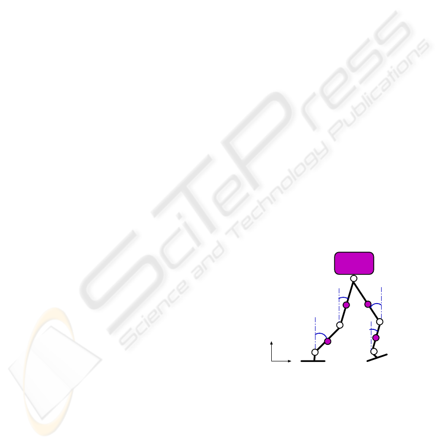
β
1
α
1
α
2
β
2
X
Z
O
m
1
m
2
m
5
m
4
x
b
y
b
x
e
y
e
m
3
Figure 1: The link model of the humanoid robot.
2 STABILITY CALCULATION
In order to evaluate dynamic stability, we use the
ZMP principle. The ZMP is the point where the
influence of all forces acting on the mechanism can
be replaced by one single force. If the ZMP is inside
133
Yin C., Zheng D. and Xiao L. (2008).
WALKING PLANNING AND CONTROL FOR A BIPED ROBOT UPSTAIRS.
In Proceedings of the Fifth International Conference on Informatics in Control, Automation and Robotics - RA, pages 133-139
DOI: 10.5220/0001475301330139
Copyright
c
SciTePress
the support polygon, the biped robot can be stable. If
the ZMP is on the boundary of the support polygon,
the robot will fall down or have a trend of falling
down. If the computed ZMP is outside the support
polygon, then the robot will fall down and in this
case, the computed ZMP is called fictitious ZMP.
The link model of the humanoid robot is shown in
Figure 1.
The projection of position vector of computed
ZMP can be computed by the following equations:
)1(
)(
)(
5
1
5
1
5
1
5
1
∑
∑∑∑
=
===
+
+−+
=
i
ii
i
iy
i
iii
i
iii
zmp
gzm
Mzxmxgzm
x
&&
&&
&&
)2(
)(
)(
5
1
5
1
5
1
5
1
∑
∑∑∑
=
===
+
+−+
=
i
ii
i
ix
i
iii
i
iii
zmp
gzm
Mzymygzm
y
&&
&&
&&
where
i
m
is mass of every links, (
i
x
,
i
y
,
i
z
) is the
coordinate of the mass center of the links,
(, )
T
ix iy
MM
is the moment vector.
If the ZMP is inside the support polygon and the
minimum distance between the ZMP and the
boundaries of support polygon is large, then the
biped will be in high stable, and this distance is
called the stability margin. We can know the
situation of walking stability from the stability
margin.
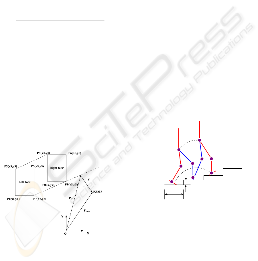
Figure 2: The relationship between FZMP and support
polygon.
As shown in Figure2, if the ZMP is outside the
support polygon, i.e. FZMP, the norm of
vector
s
represents the shortest distance between
FZMP and the edges of the support polygon. This
edge is called rotation edge. The direction of
vector
s
is the rotation direction of the robot.
3 GAIT PLANNING OF ANKLE
WHEN GOING UPSTAIRS
In order to simplify research process we first discuss
how to get ankle trajectory and hip trajectory. Then
the knee trajectory could be got by kinematics. Here
we take the left foot for example and the right foot is
similar only with a delay of half cycle. The link
model we used is shown in Figure 3.
3.1 Gait Planning of Ankle
According to the walking procedure of human, we
suppose that the walking cycle is
c
T
,
c
kTt =
is the
k
th cycle begins with the moment when the left
foot is just apart from the ground and ends with the
left foot gets into contact with the ground;
dcc
TkTtkT
+
≤
<
is double support phase, during
which the sole is rotated about toes, and the center of
gravity moving forwards; the swing foot reaches the
highest point when
nc
TkTt
+
=
.
),,(
hhh
zx
θ
),,(
fsfsfs
zx
θ
),,(
fefefe
zx
θ
H
L
l
a
l
b
Figure 3: The model of the humanoid robot going upstairs.
We get the key point
)(),( tztx
ff
of ankle in
plane
XOZ
as follows:
ICINCO 2008 - International Conference on Informatics in Control, Automation and Robotics
134

2
2(1cos)sin
2
(3)
2 ( 1) (1 cos ) sin ( 1)
2( 1) ( 1)
2( 2) ( 2)
fs c
fs a f f fs c d
fs cn
f
fs b f f fe c
fs cd
fs c
xLk tkT
xLkl h tkTT
xLkL tkTT
x
xLk l h tkT
xLk tkTT
xLk tkT
θθ
θθ
+=
⎧
⎪
++− + =+
⎪
⎪
++ =+
⎪
⎪
=
⎨
++−− − =+
⎪
⎪
++ =++
⎪
⎪
++ =+
⎪
⎩
2
2cossin
2
(4)
2( 1) cos sin ( 1)
2( 1) ( 1)
2( 2) ( 2)
fs f c
fs f fs a fs c d
fs f c n
f
fs f fe b fe c
fs f c d
fs f c
zHkh tkT
zHkh l tkTT
zHkhH tkTT
z
zHk h l tkT
zHk h tkTT
zHk h tkT
θθ
θθ
⎧
++ =
⎪
⎪
++ + =+
⎪
⎪
+++ =+
⎪
=
⎨
+++ + =+
⎪
⎪
+++ =++
⎪
⎪
+++ =+
⎪
⎩
where
a
l
is the distance between tiptoe and the centre
of gravity of sole;
b
l
is the distance between heel
and the centre of gravity of sole;
f
h
is the height of
heel and
n
T
is the time when the robot just walks
through a step.
The key point of the angle between sole and
ground can be denoted as follows:
0
0(5)
(1)
0(1)
c
fs c d
fcn
fe c
cd
tkT
tkTT
tkTT
tk T
tk TT
θ
θ
θ
⎧
=
⎪
=+
⎪
⎪
==+
⎨
⎪
=+
⎪
⎪
=+ +
⎩
Since the whole sole of the right foot is in
contact with the ground at
c
tkT=
and
(1)
cd
tk TT=+ +
, the following derivative
constraints must be satisfied.
()0
(( 1) ) 0
fc
fcd
xkT
xk TT
=
⎧
⎪
⎨
++=
⎪
⎩
&
&
(6)
()0
(( 1) ) 0
fc
fcd
zkT
zk TT
=
⎧
⎪
⎨
++=
⎪
⎩
&
&
(7)
()0
(( 1) ) 0
fc
fcd
kT
kTT
θ
θ
⎧
=
⎪
⎨
++=
⎪
⎩
&
&
(8)
3.2 Gait Planning of Hip
We assume that the robot is decelerated in double
support phase and accelerated in single support
phase and the acceleration in direction of
x
-axis
and
z -axis are
xh
a
and
zh
a
respectively. The
distance between the hip and the ankle of supporting
leg is
s
x
at the beginning of the double support
phase and
e
x
at the end of the double support phase.
The changes in the direction of
z
-axis are
s
z
and
e
z
at the beginning and end of the double support
phase respectively. Then the trajectory of hip can be
expressed like this:
It must satisfy the following constraints:
The derivative constraints
() (1)
() (1)
hc h c
hc h c
x
kT x k T
x
kT x k T
=+
⎧
⎨
=+
⎩
&&
&& &&
and
() (1)
() (1)
hc h c
hc h c
zkT zk T
zkT zk T
=+
⎧
⎨
=+
⎩
&&
&& &&
must be satisfied.
max
()
h
zt h
≤
,
max
h
is the maximum height of
hip;
max 1 2
f
hllh
=
++
,
12
,ll
are the length of
thigh and shin respectively,
f
h
is the height
of ankle.
min
()
h
zt h≥
,
min
h
is the minimum height of
hip and it’s value can be set according to the
process of human walking.
221/2
12
{[ () ()] [ () ()]}
ha ha
x
txt ztzt ll
−
+− ≤+
WALKING PLANNING AND CONTROL FOR A BIPED ROBOT UPSTAIRS
135

2
2
2
() (9)
2( 1) ( 1)
2( 1) ( 1)
2( 1) ( 2)
hs c
hsxh cd
hcn
h
hexh c
he cd
hs c
xLkx tkT
xLkxat tkTT
xLkL tkTT
xt
xLk xat tkT
xLk x tkTT
xLk x tkT
++ =
⎧
⎪
+++ =+
⎪
⎪
++ =+
⎪
=
⎨
++−− =+
⎪
⎪
++− =++
⎪
⎪
+++ =+
⎩
2
2
2
() (10)
2( 1) ( 1)
2( 1) ( 1)
2( 1) ( 2)
hs c
hszh cd
hcn
h
hezh c
he cd
hs c
zHkz tkT
z Hkz at tkT T
zHkH tkTT
zt
zHk zat tkT
zHk z tkTT
zHk z tkT
++ =
⎧
⎪
+++ =+
⎪
⎪
++ =+
⎪
=
⎨
++−− =+
⎪
⎪
++− =++
⎪
⎪
+++ =+
⎩
4 STABILITY CALCULATION
The maximum region enclosed by two soles’
projection on the ground is called the stable region,
as shown in Figure 4.
Lef t f oot
Ri ght f oot
A1 ( x
A1 ,
y
A1 ,
z
A1
)
A2 ( x
A2 ,
y
A2 ,
z
A2
)
A3 ( x
A3 ,
y
A3 ,
z
A3
)
A4 ( x
A4 ,
y
A4 ,
z
A4
)
Η
L12
L12
'
θ
ZMP
Figure 4: Stable region when going upstairs.
The equations of projection of
line
12
A
A
and
34
A
A
can be got:
121
'
12 1 2 1
()
:()
0
AAA
AAA
x
xxxt
lyy yyt
z
=+ −
⎧
⎪
=+ −
⎨
⎪
=
⎩
(11)
343
'
34 3 4 3
()
:()
0
AAA
AAA
x
xxxt
lyy yyt
z
=+ −
⎧
⎪
=+ −
⎨
⎪
=
⎩
(12)
than the stable region can be expressed as follows:
max 1, 2
min 1, 2
max 1, 2
min 1, 2
'
12
'
34
max( )
min( )
max( )
min( )
QQ a
QQ b
QQ m
QQ m
x
xx l
xxxl
yyyl
yyyl
l
l
=+
⎧
⎪
=−
⎪
⎪
=+
⎪
⎨
=−
⎪
⎪
⎪
⎪
⎩
(13)
We can get the distances between ZMP and
every boundary of stable region easily and the
stability margin can be expressed as:
max, min max min 12 34
min( , , , , ) (14)
xx y y
d d d d dl dl
γ
=
5 MAINTAIN STABILITY BY
ENLARGING SUPPORT
POLYGON
As we said above, if the computed ZMP is outside
the support polygon, the robot cannot be in dynamic
stable and has the trend of falling down. In this case
we can enlarge the support polygon to maintain
stability.
As shown in Figure 5, the changed angle
*
f
α
of
moving direction of the foot is determined by the
following equation:
*1
cos
f
es
es
α
−
⋅
=
⋅
(15)
ICINCO 2008 - International Conference on Informatics in Control, Automation and Robotics
136
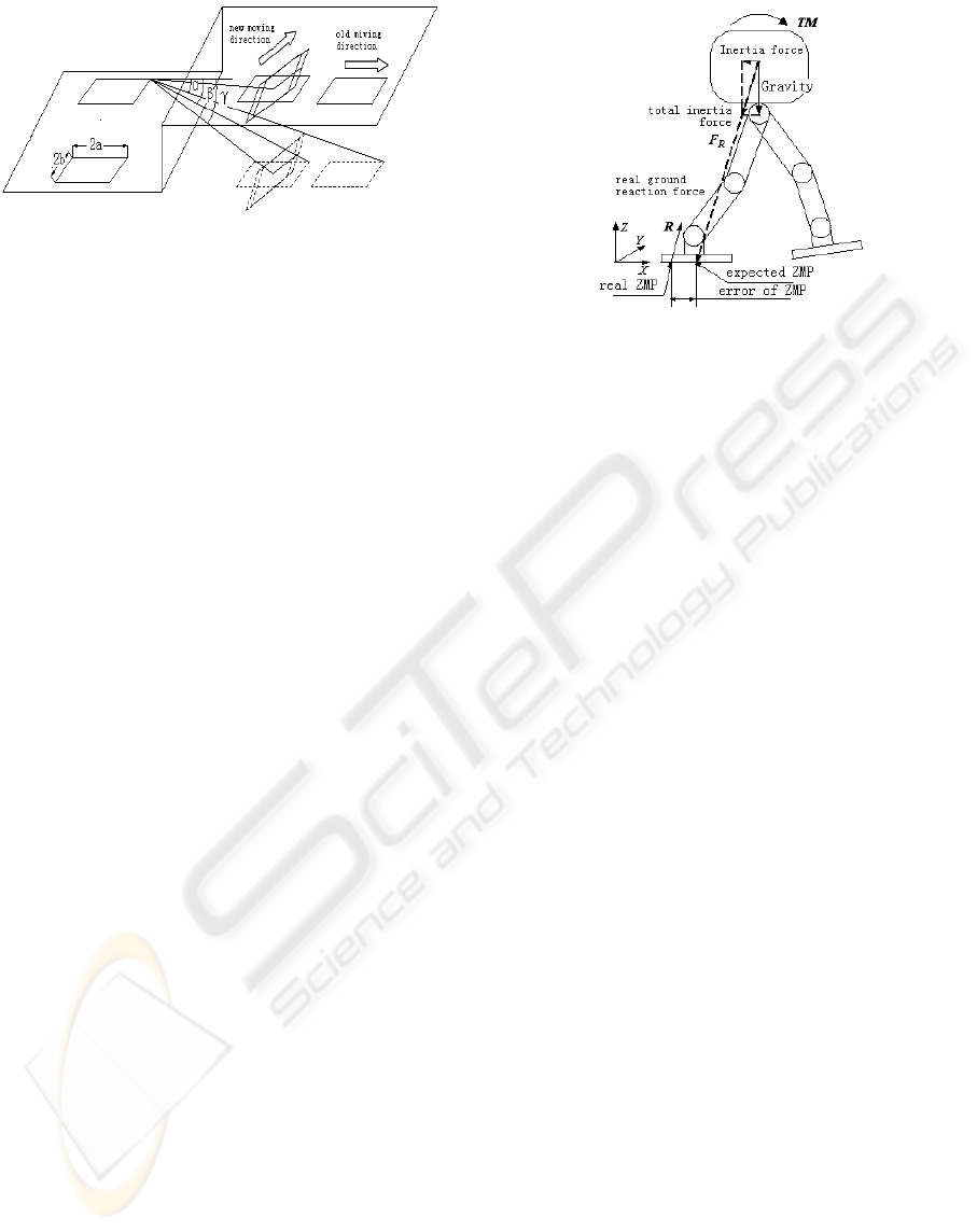
Figure 5: The determination of foot landing position.
where
e
is the normal vector of planed moving
direction and
s
is the changed vector. If the gradient
of step is
θ
and the distance between the feet is
d
,
then the foot moving distance
*
f
l
relative to planed
landing position is determined by the following
formula:
()
()
()
2
**22 2 *
2
22 2 *
tan( ) cos 3 sin cos( )
cos 3 sin sin( )
f
lldb b
ldb a
αβ θ θ γα
θθγα
⎡⎤
=− ++ −−
⎣⎦
⎡⎤
−++ −−
⎣⎦
(16)
where
β
is the original angle of foot and
γ
is the
changed angle of foot centre.
a
,
b
express half of
the foot’s long and width respectively.
6 CONTROL STRATEGY
If the computed ZMP is inside the support polygon
then the robot can be in stable. But, the error
between the computed ZMP and the designed ZMP
is unavoidable. It means that the stability condition
is not the best and we can make the robot more
stable. Our control system (the left part) shown in
Figure 7 can optimize the position of actual ZMP to
enlarge the stable margin.
As shown in Figure 6, the inertial force
R
F
and
ground reaction force
R
are not in the same line. In
this case
R
F
,
R
and the error of ZMP form a moment
which makes the robot roll. So it is necessary to
reduce the error to diminish the moment. The rolling
moment can be depicted like this
TM = (DZMP
-
AZMP)×
R
F
(17)
where DZMP means desired ZMP; AZMP means
actual ZMP.
We can obtain the error of ZMP (
Z
M
P
Δ
)
according to the desired ZMP and the actual ZMP.
The gait adjustment parameter
θ
Δ
can be got using
inverse kinematics.
Figure 6: Error of ZMP.
Z
M
P
KKKKKZMPK
T
T
Δ=Δ=
ΔΔΔΔΔ=Δ
],,,,[
],,,,[
21321
21321
ββααα
ββαααθ
(18)
where
K
is the adjustment coefficient matrix by
experience.
If there is an external disturbance, the computed
ZMP may be out of the support polygon and the
robot may tip over, at this moment the control
system (the right part) will take action.
Two important parameters can be got according
to the definition of FZMP, i.e. the distance between
FZMP and the rotation edge and the rotation
direction. We can also get the change of the angle of
link
θ
Δ
by the sensor fitted at the link. The
emergency-coping strategies such as enlarging the
support polygon, moving the upper body and
contacting with surrounding by hands can be used to
make the FZMP located in the support polygon and
maintain the stability of the robot. Whereas, in some
cases one method along may be unrealistic, two or
three methods can be combined.
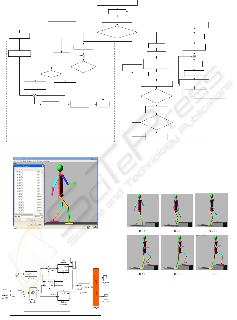
7 SIMULATION
We have constructed a simulator of a humanoid
robot by using dynamic analysis software package
ADMAS and the control system is built in Matlab.
This allows us to analyze the joint torque, the
change of ZMP, etc. The simulator built in ADMAS
is shown in Figure 8.
WALKING PLANNING AND CONTROL FOR A BIPED ROBOT UPSTAIRS
137
Gai t pl anni ng of ankl e and hi p
Fuzzy control
Support polygon calculation
is in the support
po lygon or not
Actual ZMP£½
FZMP£½
Model of humanoid robot
Desigred
ZMP
>thre
shold value
Walk s tab ly
Parameter of joint
adjustment
Parameter of joint
Gte the valve of ||s||
The distance between
FZMP and roll edge and
the rotation derection
Change of joint's angle
Satify the constrants
of foot location
Satify the
constrants of
upper body
YES
Upper body lean
NO
Touch other things
by hand
YES
YES NO
£-
£«
YES NO
NO
K×
is in the support polygon
is out of the support polygon
|||| ZMPΔ
Inverse kinematics
>0
ZMPΔ
θ
Δ
YES
Parameter of joint
adjustment
θ
Δ−
NO
K×
θ
Dynamics
£«
£«
£«
Humanoid robot
i
θ
Δ
Model of humanoid robot
Parameter of joint
Inverse kinematics
i
θ
£«
£-
iii
θθθ
Δ+=
Forward kinematics
Real location of foot
ha PP 、
cP
ff zx ,
cP
cP
cP
Rrprogram of the
trajectory of foot
aP
α
Δ
calculate actul
ZMP
Angle sensor
cP
cP
Figure 7: The control strategy.
Figure 8: The ADMS model of humanoid robot.
The structure of control system based on
Matlab/simulink is shown as follows:
Figure 9: The structure of control system.
We simulate the procedure of walking up and down
stairs with a height of 0.2m and a width of 0.6m.
The pictures of series of walking upstairs are shown
in Figure 10 at the time of 0.0s, 0.2s, 0.4s, 0.6s, 0.8s
and 1.0s.
Figure 10: Series of walking upstairs.
The velocity and acceleration of ankle and hip
are given in Figure 11 and 12 respectively. The
x-axis represents time and the y-axis represents the
velocity of ankle and hip. The red real line is
velocity and the blue dashed is acceleration.
ICINCO 2008 - International Conference on Informatics in Control, Automation and Robotics
138
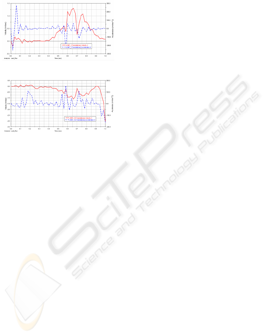
Figure 11: Velocity and acceleration of ankle.
Figure 12: Velocity and acceleration of hip.
Figure 11 shows that the maximum velocity
happens when the swing foot is descending and it is
consisdent with the real walking process of human.
It also shows that the velocity and acceleration are
close to zero at the time of 1.0s and the slope is
getting smaller when the time is getting nearer to
1.0s. We all know that the landing acceleration of
ankle is very important for the stability of robot. If
the acceleration is too big, the impact force between
robot and ground may be very large and the robot
may become unstable. So in our simulation, the
impact force is very small and the robot can walk
stably. It shows that the strategy described above
works.
8 CONCLUSIONS
Biped robots have better mobility than wheeled
robots but tip over easily, so the walking stability is
even more important. When going upstairs the
stability problem is especially crucial and the
research is far from enough. In order to make the
robot go upstairs stably, it is necessary to have an
efficient control strategy to scout and make
adjustment on time. In this paper, we propose a
method to plan a walking pattern and the way of
calculating the stable region and stability margin is
also presented. The stability maintenance method of
enlarging support polygon is given out. The
optimization control strategy which is proved to be
useful by numerical simulation is proposed.
REFERENCES
Huang, Q., Kajita, S., Koyachi, N., Kaneko, K., Yokoi, K.,
Arai, H., Komoriya, K., Tanie, K., 1999. A High
Stability, Smooth Walking Pattern for a Biped Robot.
Proceedings of IEEE International Conference
Robotics and Automation.
Kaneko, K., Kajita, S., Kanehiro, F., Yokoi, K., Fujiwara,
K., Hirukawa, H., Kawasaki, T., Hirata, M., Isozumi,
T., 2002. Design of Advanced Leg Module for
Humanoid Robotics Project of METI. Proceedings of
IEEE International Conference on Robotics &
Automation.
Konno, A., 2002. Design And Development of the Biped
Prototype Robian. Proceedings of IEEE International
Conference on Robotics & Automation.
Pfeiffer, F., Loeffer, K., Gienger, M., 2002. The Concept
of Jogging JOHNNIE. Proceedings of IEEE
international conference on robotics & Automation.
Kajita, S., Kanehiro, F., Kaneko, K., Fujiwara, K., Harada,
K., Yokoi. K., Hirukkawa, H., 2003. Biped Walking
Patern Generation By Using Preview Control of
Zero-Moment Point. Proceedings of IEEE
International Conference on Robotics &Automation.
Stojic, R., Chevallereau, C., 2000. On the Stability of
Biped with Point Foot-Ground Contact. Proceedings
of IEEE International Conference on Robotics
&Automation.
Vukobratovic, M., 1990. Biped Locomotion: Dynamics,
Stability, Control And Application. Spring Verlag,
Berlin.
Vukobratovic, M., Borovac, B., 2004. Zero-Moment
Point-Thirty Five Years of Its Life. International
Journal of Humanoid Robotics Vol. 1.
Yoneda, K., Hirose, S., 1996. Tumble Stabilit Criterion of
Integrated Locomotion and Manipulation. Proceedings
of IEEE International Conference on Intelligent Robot
and Systems.
Gowami, A., 1999. Postural Stability of Biped Robots and
the Foot-Rotation Indicator (FRI) Point. The
International Journal of Robotics Research, vol.18.
Yin, C.B., Albert, A., 2005. Stability Maintenance of a
Humanoid Robot under Disturbance with Fictitious
Zero-Moment Point. IEEE/RSJ International
Conference on Intelligent Robots and Systems.
Narikiyo, T., Ohmiya, M., 2006. Control of a planar space
robot: Theory and experiments. Control Engineering
Practice,Vol. 14, Issue 8.
Kajita, S., Nagasaki, T., Kaneko, K., Tanie, K., 2004. A
Hop towards Running Humanoid Biped. Proceedings
of IEEE International Conference Robotics and
Automation
WALKING PLANNING AND CONTROL FOR A BIPED ROBOT UPSTAIRS
139
