
RECURSIVE AND BACKWARD REASONING IN THE
VERIFICATION ON HYBRID SYSTEMS
Stefan Ratschan
Institute of Computer Science, Czech Academy of Sciences, Prague, Czech Republic
Zhikun She
LMIB and School of Science, Beihang University, Beijing, China
Keywords:
Hybrid Systems, Verification, Constraint Propagation.
Abstract:
In this paper we introduce two improvements to the method of verification of hybrid systems by constraint
propagation based abstraction refinement that we introduced earlier. The first improvement improves the
recursive propagation of reachability information over the regions constituting the abstraction, and the second
improvement reasons backward from the set of unsafe states, instead of reasoning forward from the set of
initial states. Detailed computational experiments document the usefulness of these improvements.
1 INTRODUCTION
Safety verification of hybrid systems is the problem
of verifying that for a given hybrid system no trajec-
tory that starts in an initial state ever reaches an unsafe
state. Abstraction refinement approaches this prob-
lem by iteratively refining an overapproximation of
the hybrid system (the abstraction) that is constructed
in such a way that the safety of the abstraction im-
plies the safety of the concrete system. In our method
of constraint propagation based abstraction refine-
ment (Ratschan and She, 2007) the abstraction is built
by decomposing the state-space into hyper-rectangles
(boxes) and using a constraint solver to test, which of
these boxes might contain an initial/unsafe state, and
which box might be reachable from another box.
In this paper, we introduce two improvements to
the method: recursive reasoning and backward rea-
soning. Recursive reasoning improves the way the
method removes elements from boxes for which it can
prove that they are not reachable from an initial state.
The original method argues that a point in a box is
not reachable from another box, if it is not reachable
from a point on the common boundary. In this pa-
per we strengthen this condition using a convenient
over-approximation of the requirement that this com-
mon point on the boundary again has to be reachable.
Backward reasoning uses the observation that we can
remove not only elements from boxes for which we
can prove that they are not reachable from an initial
state, but also elements for which we can prove that
they do not lead to an unsafe state.
There are various other methods for the verifica-
tion of hybrid systems that use a decomposition of the
state space into boxes (Preußig et al., 1999; Kloet-
zer and Belta, 2006). Another paper (Frehse et al.,
2006) employs backward reasoning in a more coarse-
grained manner than in this paper, computing over-
approximations of increasingly precise forward and
backward reach sets.
The content of the paper is as follows: In Sec-
tion 2 we review our hybrid systems formalism, and
in Section 3 we review our verification method and
discuss properties of the underlying constraint solv-
ing technique; in Sections 4 and 5 we introduce the
first improvement to our verification method, and in
Section 6 our second improvement and the combina-
tion of the two improvements; in Section 7 we present
some computational experiments, and in Section 8 we
conclude the paper.
2 VERIFICATION OF HYBRID
SYSTEMS
Hybrid systems are systems with continuous and dis-
crete state variables. In this paper, we briefly recall
our formalism for modeling hybrid systems (Ratschan
and She, 2007).
We use a set S to denote the modes of a hybrid
65
Ratschan S. and She Z. (2008).
RECURSIVE AND BACKWARD REASONING IN THE VERIFICATION ON HYBRID SYSTEMS.
In Proceedings of the Fifth International Conference on Informatics in Control, Automation and Robotics - SPSMC, pages 65-71
DOI: 10.5220/0001475500650071
Copyright
c
SciTePress

system, where S is finite and nonempty. I
1
,...,I
k
⊆ R
are compact intervals over which the continuous vari-
ables of a hybrid system range. Φ denotes the state
space of a hybrid system, i.e., Φ = S × I
1
× ··· × I
k
.
Definition 1. A hybrid system H is a tuple
(Flow,Jump, Init,Unsafe), where Flow ⊆ Φ × R
k
,
Jump ⊆ Φ× Φ, I ⊆ Φ, and Unsafe ⊆ Φ.
Informally speaking, the predicate Init specifies
the initial states of a hybrid system and Unsafe the
states that should not be reachable from an initial
state. The relation Flow specifies how the system may
developcontinuously by relating each state to the pos-
sible corresponding derivatives, and Jump specifies
how H may change states discontinuously by relating
each state to its possible successor states. Formally,
the behavior of H is defined as follows:
Definition 2
. A flow of length l ≥ 0 in a mode s ∈ S
is a function r : [0,l] → Φ such that the projection of
r to its continuous part is differentiable and for all
t ∈ [0,l], the mode of r(t) is s. A trajectory of H is a
sequence of flows r
0
,...,r
p
of lengths l
0
,... , l
p
such
that for all i ∈ {0,..., p},
1. if i > 0 then (r
i−1
(l
i−1
),r
i
(0)) ∈ Jump, and
2. if l
i
> 0 then (r
i
(t), ˙r
i
(t)) ∈ Flow, for all t ∈ [0, l
i
],
where ˙r
i
is the derivative of the projection of r
i
to
its continuous component.
Definition 3
. A (concrete) counterexample of a hy-
brid system H is a trajectory r
0
,...,r
p
of H such that
r
0
(0) ∈ Init and r
p
(l) ∈ Unsafe, where l is the length
of r
p
. H is safe if it does not have a counterexample.
We use the following constraint language to de-
scribe hybrid systems and corresponding safety veri-
fication problems. The variable s ranges over S and
the tuple of variables ~x = (x
1
,... , x
k
) ranges over
I
1
× ··· × I
k
, respectively. In addition, to denote the
derivatives of x
1
,... , x
k
we use the tuple of variables
˙
~x = ( ˙x
1
,... , ˙x
k
) that ranges over R
k
, and to denote the
targets of jumps, we use the primed variable s
′
and
the tuple of variables~x
′
= (x
′
1
,... , x
′
k
) that range over
S and I
1
× · · · × I
k
, respectively. Constraints are arbi-
trary Boolean combinations of equalities and inequal-
ities over terms that may contain function symbols,
such as +, ×, exp, sin, and cos.
We assume in the remainder of the text that a hy-
brid system is described by our constraint language.
That means, the flows of a hybrid system are given
by a constraint Flow(s,~x,
˙
~x), the jumps are given by a
constraint Jump(s,~x,s
′
,~x
′
), the initial states are given
by a constraint Init(s,~x), and a constraint Unsafe(s,~x)
describes the unsafe states. To simplify notation, we
do not distinguish between a constraint and the set it
represents.
Example 1. Consider the following simple hybrid
system with the modes m
1
,m
2
and the continuous
variables x
1
,x
2
which both range over the interval
[0,2], i.e, Φ = {m
1
,m
2
} × [0, 2] × [0, 2].
The set of initial states are given by the
Init(s, (x
1
,x
2
)) = (s = m
1
∧ x
1
= 0 ∧ x
2
= 0). The
constraint Unsafe(s,(x
1
,x
2
)) = (x
1
> 1.5∧ x
2
= 1.5)
describes the set of unsafe states. The hybrid sys-
tem can switch modes from m
1
to m
2
if x
2
= 1, i.e.,
Jump(s,(x
1
,x
2
),s
′
,(x
′
1
,x
′
2
)) = (s = m
1
∧ x
2
= 1) →
(s
′
= m
2
∧ x
′
1
= x
1
∧ x
′
2
= x
2
) . The continuous be-
havior is described by constants. In addition, for a
flow in mode m
1
, the constraint 0 ≤ x
1
≤ 1 must hold.
The corresponding flow constraint is
Flow(s,(x
1
,x
2
),(˙x
1
, ˙x
2
)) =
(s = m
1
→ ( ˙x
1
= 1 ∧ ˙x
2
= 1 ∧ 0 ≤ x
1
≤ 1)) ∧
(s = m
2
→ ( ˙x
1
= 1 ∧ ˙x
2
= −1)) .
Note that the constraint 0 ≤ x
1
≤ 1 in flow forces a
jump from mode m
1
to m
2
if x
1
becomes 1.
Obviously, this hybrid system is safe.
3 FORWARD SEARCH BASED
ABSTRACTION REFINEMENT
In this section, we review our previous ap-
proach (Ratschan and She, 2007) for verifying safety
of hybrid systems using constraint propagation based
abstraction refinement.
We abstract to systems of the following form:
Definition 4
. A discrete system over a finite set S is
a tuple (Trans,Init, Unsafe) where Trans ⊆ S × S and
Init ⊆ S, Unsafe ⊆ S. We call the set S the state space
of the system.
In contrast to Definition 1, here the state space is a
parameter. This will allow us to add new states to the
state space during abstraction refinement.
Definition 5
. A trajectory of a discrete system
(Trans, Init, Unsafe) over a set S is a function r :
{0, . . . , p} 7→ S such that for all t ∈ {1, . . . , p}, (r(t −
1),r(t)) ∈ Trans. The system is safe if and only if there
is no trajectory from an element of Init, to an element
of Unsafe.
When we use abstraction to analyze hybrid sys-
tems, the abstraction should over-approximate the
concrete system in a conservative way: if the abstrac-
tion is safe, then the original system should also be
safe. If the current abstraction is not yet safe, we re-
fine the abstraction, that is, we include more informa-
tion about the concrete system into it. This results in
Algorithm 1.
ICINCO 2008 - International Conference on Informatics in Control, Automation and Robotics
66

Algorithm 1: Abstraction Refinement.
Require: a hybrid system H described by constraints
Ensure: “safe”, if the algorithm terminates
let A be a discrete abstraction of the hybrid system
represented by H
while A is not safe do
refine the abstraction A
end while
In order to implement this algorithm, we need to
fix the state space of the abstract system. Here we use
pairs (s, B), where s is one of the modes {s
1
,... , s
n
}
and B is a hyper-rectangle (box), representing subsets
of the concrete state space Φ. Together with an ab-
stract state, we store the information whether it is ini-
tial or unsafe and the information from which other
states it is reachable. We call such information the
marks of the state. For the initial abstraction we use
the state space {(s
i
,{~x | (s
i
,~x) ∈ Φ}) | 1 ≤ i ≤ n},
where all states are marked as initial, and unsafe, and
all transitions between states are possible.
For refining the abstraction, we split a box into
two pieces, replace one abstract state by two, and in-
clude more information from the concrete system into
the abstract one by removing unreachable elements
from the boxes, removing superfluous marks from the
new abstract states, and removing unreachable states
from the abstraction.
To remove unreachable elements from the boxes
representing the abstraction, we use a constraint that
formalizes when an element of the concrete state
space might be reachable, and then remove elements
that do not fulfill this constraint. In order to do this,
for a box B = [x
1
,x
1
] × · · · × [x
k
,x
k
], we let its j-th
lower face be [x
1
,x
1
]× ··· × [x
j
,x
j
]× ···× [x
k
,x
k
] and
its j-th upper face be [x
1
,x
1
] × · · · × [x
j
,x
j
] × · · · ×
[x
k
,x
k
]. Two boxes are non-overlapping if their in-
teriors are disjoint.
Now observe that a point in a box B is reachable
only if it is reachable either from the initial set via
a flow in B, from a jump via a flow in B, or from a
neighboring box via a flow in B. We will now formu-
late constraints corresponding to each of these condi-
tions. Then we can remove points from boxes that do
not fulfill at least one of these constraints.
The approach can be used with any constraint that
describes that~y can be reachable from~x via a flow in
B and mode s, for example, the one introduced in our
previous publications (Ratschan and She, 2006). We
denote the used constraint by Reach
B
(s,~x,~y). Thus,
the above three possibilities for reachability allow us
to formulate the following theorem:
Theorem 1. For a set of abstract states B , a pair
(s
′
,B
′
) ∈ B and a point~z ∈ B
′
, if (s
′
,~z) is reachable
and z is not an element of the box of any other abstract
state in B , then
Ifl
B
′
(s
′
,~z) ∨
_
(s,B)∈B
Jfl
B,B
′
(s,s
′
,~z)
∨
_
(s,B)∈B ,s=s
′
,B6=B
′
Bfl
B,B
′
(s
′
,~z)
where Ifl
B
′
(s
′
,~z), Jfl
B,B
′
(s,s
′
,~z), and Bfl
B,B
′
(s
′
,~z) de-
note the following three constraints, respectively:
• ∃~x ∈ B
′
[Init(s
′
,~x) ∧ Reach
B
′
(s
′
,~x,~z)],
• ∃~x ∈ B∃~x
′
∈ B
′
[Jump(s,~x, s
′
,~x
′
) ∧
Reach
B
′
(s
′
,~x
′
,~z)]
• ∃~x ∈ B ∩ B
′
[[∀faces F of B
′
[~x ∈ F ⇒ in
F
s
′
,B
′
(~x)]] ∧
Reach
B
′
(s
′
,~x,~z)].
Here, in
F
s
′
,B
′
(~x) = ∃ ˙x
1
,... , ∃ ˙x
k
[F(s
′
,~x, ( ˙x
1
,... , ˙x
k
)) ∧
˙x
j
≥ 0], if F is the j-th lower face of B
′
, and if
F is the j-th upper face of B
′
, incoming
F
s
′
,B
′
(~x) =
∃ ˙x
1
,... , ∃ ˙x
k
[F(s
′
,~x,( ˙x
1
,... , ˙x
k
)) ∧ ˙x
j
≤ 0].
We denote the main constraint of Theorem 1 by
reach
B ,B
′
(s
′
,~z). If we can prove that a certain point
does not fulfill this constraint, we know that it is not
reachable. For now, we assume that we have an al-
gorithm (a pruning algorithm) that takes such a con-
straint, and an abstract state (s
′
,B
′
) and returns a sub-
box of B
′
that still contains all the solutions of the
constraint in B
′
. Since the constraint reach
B ,B
′
(s
′
,~z)
depends on all current abstract states, a change of B
′
might allow further pruning of other abstract states.
So we can repeat pruning until a fixpoint is reached.
Given a set of abstract states B , we denote the result-
ing fixpoint by Prune
H
(B ).
Now we remove the initial mark from an abstract
state (s
′
,B
′
) if we can disprove Ifl
B
′
(s
′
,~z
′
) in The-
orem 1 (i.e., if the pruning algorithm returned the
empty box for this constraint), and we remove the un-
safe mark of an abstract state state (s
′
,B
′
) if we can
disprove the constraint ∃~x ∈ B Unsafe(s,~x). More-
over, we remove a transition from (s,B) to (s
′
,B
′
) if
we can disprove both Bfl
B,B
′
(s
′
,~z
′
) and Jfl
B,B
′
(s,s
′
,~z
′
)
from Theorem 1. As already mentioned, after recom-
puting the marks, we remove all abstract states from
the abstraction that are not reachable. It is easy to
compute these, since the set of abstract states is finite.
There are several methods for implementing the
needed pruning algorithms (Benhamou and Granvil-
liers, 2006). For the domain of the real numbers,
given a constraint c and a floating-point box B, they
compute another floating-point box P(c,B) such that
P(c,B) ⊆ B (contractance), and such that P(c, B) con-
tains all solutions of c in B. Existential quantifiers and
disjunctions can be handled by slight extensions (for
disjunctions we take the box union ⊎).
RECURSIVE AND BACKWARD REASONING IN THE VERIFICATION ON HYBRID SYSTEMS
67

Such pruning algorithms P usually have the mono-
tonicity property that for a constraint c, and boxes B
and B
′
with B
′
⊆ B, P(c,B
′
) ⊆ P(c, B). Moreover, in
practice, if B
′
⊆ B then P(c, B
′
) is often much smaller
than P(c, B). We will exploit this in the improvement
of our method described in the next section. In ad-
dition, it pays off to distribute disjunctions over con-
junctions:
Lemma 1
. For constraints c
1
,... , c
n
,d and a box B,
P(∨
i∈{1,...,n}
(c
i
∧ d),B) ⊆ P((∨
i∈{1,...,n}
c
i
) ∧ d, B)
Proof. For each i ∈ {1, . . . ,n}, P(c
i
∧
d,B) ⊆ P((∨
i∈{1,...,n}
c
i
) ∧ d, B). Thus,
⊎
i∈{1,...,n}
P(c
i
∧ d,B) ⊆ P((∨
i∈{1,...,n}
c
i
) ∧ d,B).
Since P(∨
i∈{1,...,n}
(c
i
∧d), B) = ⊎
i∈{1,...,n}
P(c
i
∧d, B),
the lemma holds.
4 RECURSIVE PRUNING
In this section we introduce the first improvement
to the verification method described in Section 3.
Throughout the rest of the paper we assume an ab-
straction consisting of a set of abstract states B . The
improvement introduced in this section aims at prun-
ing more unreachable states from B by improving the
recursive propagation of reachability information for
flows from one box to the next.
We consider the pruning of an abstract state
(s
′
,B
′
) ∈ B . The constraint Bfl
B,B
′
(s
′
,~z) defined
within Theorem 1 models the fact that a certain point
~z in the box B
′
is reached from a neighboring box B
of B
′
via a flow in B
′
. This flow reaches~z through a
common point~x ∈ B∩ B
′
(see Figure 1).
z
x
B
′
B
Figure 1: Recursive Pruning.
The basic idea upon which we build in this section
is to strengthen this constraint by requiring that also~x
be reachable in the neighboring box B. Naively, this
could be done by adding the constraint reach
B ,B
(s
′
,~x)
to the constraint Bfl
B,B
′
(s
′
,~z). However, since
Bfl
B,B
′
(s
′
,~z) is itself a part of reach
B ,B
′
(s
′
,~x), this
would result in an infinitely large constraint due to
recursion. One could make the constraint finite, by
bounding the recursion, but this still would result in
a very large constraint. We avoid this, by observ-
ing that the neighboring box B is already the result
of pruning wrt. reach
B ,B
(s
′
,~x). However, a part of
this information is lost because we first prune B and
only then take the intersection B∩B
′
(i.e., we compute
P(reach
B ,B
(s
′
,~x), B) ∩ B
′
), and we have:
Lemma 2
.
P(reach
B ,B
(s
′
,~x), B∩ B
′
) ⊆ P(reach
B ,B
(s
′
,~x),B) ∩ B
′
Proof. Due to monotonicity of constraint
propagation, P(reach
B ,B
(s
′
,~x),B ∩ B
′
) is a
subset of P(reach
B ,B
(s
′
,~x),B). Moreover,
P(reach
B ,B
(s
′
,~x), B ∩ B
′
) ⊆ P(reach
B ,B
(s
′
,~x), B
′
),
and hence P(reach
B ,B
(s
′
,~x),B ∩ B
′
) ⊆ B
′
. So
P(reach
B ,B
(s
′
,~x), B ∩ B
′
) is also a subset of the
intersection of P(reach
B ,B
(s
′
,~x), B) and B
′
.
In practice, the set on the left-hand side might
be significantly smaller than the set on the right-
hand side (i.e., than the set currently used in
the method in Section 3). So it makes sense
to compute P(reach
B ,B
′
(s
′
,~x),B ∩ B
′
) instead of
P(reach
B ,B
(s
′
,~x), B) ∩ B
′
. This means that in addition
to pruning each box in the abstraction, we could also
prune the intersection between each pair of boxes.
However, this would need a quadratical number of
prunings and stored boxes in memory.
To avoid this, we use an over-approximation
of P(reach
B ,B
(s
′
,~x),B ∩ B
′
) that is still a subset of
P(reach
B ,B
(s
′
,~x), B) ∩ B
′
. We use the information
that the boxes of our abstraction are non-overlapping
(i.e., even if two boxes intersect, they only share the
boundary but no points of the interior). This implies
that the intersection B ∩ B
′
will always be a subset
of the boundary of B—independent of the form of
the box B
′
. So one could try to use the boundary
B of B instead of the box B ∩ B
′
when computing
P(reach
B ,B
(s
′
,~x), B∩ B
′
). However, since B is not a
box and hence it cannot be an argument to the prun-
ing function, we apply the pruning function to its con-
stituent faces separately. That is, we use the constraint
that expresses a disjunction over all faces:
_
F,face of B
~x ∈ F ∧ reach
B ,B
(s
′
,~x)
and call this constraint reachbound
B ,B
(s
′
,~x). Al-
though this over-approximates P(reach
B ,B
(s
′
,~x), B ∩
B
′
), Lemma 2 still holds in analogy:
Lemma 3. P(
W
F,face of B
~x ∈ F ∧reach
B ,B
(s
′
,~x)
,B) ∩
B
′
⊆ P(reach
B ,B
(s
′
,~x), B) ∩ B
′
.
Proof. The disjunction is pruned by taking the
box union over the result of pruning each disjunct.
Since each face of B is a subset of B, due to mono-
tonicity of constraint propagation, for each face F,
P(reach
B ,B
(s
′
,~x), F) ⊆ P(reach
B ,B
(s
′
,~x), B). Hence
ICINCO 2008 - International Conference on Informatics in Control, Automation and Robotics
68

also the box union over the result of pruning each dis-
junct is a subset of P(reach
B ,B
(s
′
,~x), B), which im-
plies the lemma.
Since the constraint on the left-hand side only de-
pends on one box, we can compute the corresponding
pruning P(reachbound
B ,B
(s
′
,~x), B) only for one ab-
stract state, and store the resulting box with that ab-
stract state. Since this box encloses the set of states
where a flow might leave the abstract state, we call it
the outflow-box of the abstract state. So, instead of
B ∩ B
′
in the constraint Bfl
B,B
′
we can now take the
outflow-box of B, and due to Lemma 3 we will arrive
at a result that is at least as tight as before.
This is illustrated on an example in Figure 2,
where the dotted box is the outflow-box resulting from
a situation where the upper and left face of box B have
been pruned to the empty set, and the outflow-box is
the result of taking the union of the result of pruning
the two other faces.
z
x
B
′
B
Figure 2: Pruning Faces.
Note that splitting a box B representing a cer-
tain abstract state changes its faces. Especially, there
might be trajectories that leave the resulting boxes
through the new face along which B has been split.
Hence the outflow-box of this abstract state becomes
invalid. So we simply set the outflow-box to the
whole box B and re-compute it, the next time B is
pruned.
5 RECURSIVE PRUNING WITH
OUTGOING CONDITION
In the previous section we used the fact that within the
constraint Bfl we can exploit the information that the
common point~x ∈ B∩B
′
itself has to be reachable. In
this section we strengthen this information by observ-
ing that in order for a trajectory to be able to leave the
box B to enter the box B
′
, the vector field at x has to
point out of B.
This can be modelled by adding an additional con-
dition in the constraint reachbound
B ,B
(s
′
,~x), arriving
at
_
F,face of B
h
~x ∈ F ∧ reach
B ,B
(s
′
,~x) ∧ out
F
s
′
,B
(~x)
i
,
where out
F
s
′
,B
(~x) is equal to in
F
s
′
,B
(~x) with the inequal-
ity sign switched. Now, since reach
B ,B
(s
′
,~x) is a dis-
junction, Lemma 1 suggests to improve it by pulling
out the new conjunction of reachbound
B ,B
(s
′
,~x), ar-
riving at
_
F,face ofB
h
~x ∈ F ∧ out
F
s
′
,B
(~x) ∧ Ifl
B
(s
′
,~x)
i
∨
_
(s,B
′
)∈B
_
F,face ofB
[~x ∈ F ∧ out
F
s
′
,B
(~x)
∧ Jfl
B
′
,B
(s,s
′
,~x)]
∨
_
(s, B
′
) ∈ B
s = s
′
,B
′
6= B
_
F,face ofB
[~x ∈ F ∧out
F
s
′
,B
(~x)
∧ Bfl
B
′
,B
(s
′
,~x)]
.
We call the resulting constraint reachout
B ,B
(s
′
,~x),
and use this constraint instead to compute the outflow-
box of each abstract state.
The following examples illustrates the improve-
ment provided by reachout over reachbound: Con-
sider the differential equation ( ˙x
1
, ˙x
2
) = (1,1) with
a box B = [0,1] × [0,1] and an initial point x
0
=
(0,0). If we prune a face [1,1] × [0,1] or [0,1] × [1,1]
wrt. reachbound, we will get the point (1, 1); and
if we prune a face [0, 0] × [0, 1] or [0, 1] × [0, 0] wrt.
reachbound, we will get the point (0, 0). That is, if
we apply the pruning algorithm to reachbound and
B, we will get the full box [0,1] × [0, 1]. Only when
adding the outgoing condition, arriving at the con-
straint reachout, we can ignore trajectories moving
into the box, arriving at the point [1,1] × [1, 1].
6 BACKWARD REASONING AND
COMBINATION
As described in Section 3, in our method we remove
elements from the state space for which we can prove
that they are not reachable from an initial state. How-
ever, the task of safety verification is to prove the ab-
sence of a trajectory that starts in an initial state and
reaches an unsafe state. Hence we can also remove
elements from the state space for which we can prove
that they do not lead to an unsafe state—without de-
stroying the property that safety of the abstraction im-
plies safety of the concrete system.
For this, observe that a point might lead to an un-
safe state only if there is a flow from this point to the
unsafe set directly, or a flow from this point to a jump,
or a flow from this point to a boundary point. Hence
we can formulate an analogous version of Theorem 1:
RECURSIVE AND BACKWARD REASONING IN THE VERIFICATION ON HYBRID SYSTEMS
69

Theorem 2. For a set of abstract states B , a pair
(s
′
,B
′
) ∈ B and a point ~z ∈ B
′
, if the unsafe set is
reachable from (s
′
,~z) and~z is not an element of the
box of any other abstract state in B , then
Urev
B
′
(s
′
,~z) ∨
_
(s,B)∈B
Jrev
B,B
′
(s,s
′
,~z)
∨
_
(s,B)∈B ,s=s
′
,B6=B
′
Brev
B,B
′
(s
′
,~z),
where Urev
B
′
(s
′
,~z), Jrev
B,B
′
(s,s
′
,~z), and
Brev
B,B
′
(s
′
,~z) denote the following three constraints,
respectively:
• ∃~x ∈ B[Reach
B
(s,~z,~x) ∧ Unsafe(s,~x)],
• ∃~x ∈ B∃~x
′
∈ B
′
[Reach
B
(s,~z,~x) ∧ Jump(s,~x, s
′
,~x
′
)]
• ∃~x ∈ B ∩ B
′
[Reach
B
(s,~z,~x) ∧ [∀ faces F of B[~x ∈
F ⇒ in
F
s,B
′
(x)]]]
In a similar way as forward reasoning, backward
reasoning also allows us to update the initial/unsafe
marks and transitions of the abstraction.
Note that by using forward and backward reason-
ing in Algorithm 1 we might succeed in removing
all elements from the concrete state space. This re-
sults in an empty abstraction which is trivially safe.
Hence, Algorithm 1 can report a successful verifica-
tion in this case. However, the combination of recur-
sive pruning with backward pruning introduces addi-
tional difficulties: the outflow box is computed using
forward reasoning, and when a box is changed due to
backward reasoning, its outflow box is not valid any
more. We solve this problem by always, first apply-
ing forward pruning and then backward pruning. If
backward pruning changes the box, we apply forward
pruning again which recomputes a valid outflow box.
7 EXPERIMENTAL RESULTS
We extended our hybrid systems verification package
HSOLVER (Ratschan and She, 2004) with the two im-
provements introduced in this paper. Then we used
our problem database
1
of hybrid systems to evaluate
our improvements. The experimental results are sum-
marized in Table 1, Table 2 and Table 3 for different
versions.
We used an IBM notebook with an Intel Pentium
1.70 GHz CPU with 1024Mbytes of main memory
running Linux. The running times are in seconds and
the computations were cancelled when computation
did not terminate before three hours or the number of
the abstract states exceeded 1000. We used the default
splitting strategy of HSOLVER.
1
http://hsolver.sourceforge.net/benchmarks
Table 1: Experimental Results: I.
Forward
Example time splits
1-flow unknown
2-tanks 1.12 31
car 0.47 0
circuit 53.80 186
clock 1.99 32
convoi-1 1.06 0
convoi 2157.26 374
eco 125.24 223
focus 3.59 57
mixing 296.67 174
mutant 7286.40 742
real-eigen 0.59 2
s-focus 0.54 2
trivial-hard 0.76 26
van-der-pole (VDP) 25.42 64
Table 2: Experimental Results: II.
Backward For-Backward
Example time splits time splits
1-flow unknown 0.32 1
2-tanks 0.10 6 0.43 4
car unknown 1.05 0
circuit unknown 62.99 188
clock 35.79 327 2.00 43
convoi-1 unknown 1.65 0
convoi unknown 1847.67 300
eco unknown 18.32 52
focus 0.62 34 0.89 15
mixing 1.47 7 1.74 0
mutant unknown 8493.97 618
real-eigen unknown 0.61 0
s-focus unknown 0.44 1
trivial-hard 0.03 0 0.05 0
VDP 0.47 1 0.77 1
Comparing the forward version and backward ver-
sion, there is no clear winner, although the forward
version is successful in more cases. The reason seems
to lie in the fact that for more examples the set of ini-
tial states is smaller than the set of unsafe states.
Moreover, the experimental results show that: (1)
For most of the examples, the combined forward and
backward version use less splitting steps than both
the forward version and backward version. How-
ever, for some examples, the CPU time is worse since
in the combined version, the constraints are more
complex. Note that for some examples (e.g., circuit
and clock), the combined version needs slightly more
ICINCO 2008 - International Conference on Informatics in Control, Automation and Robotics
70
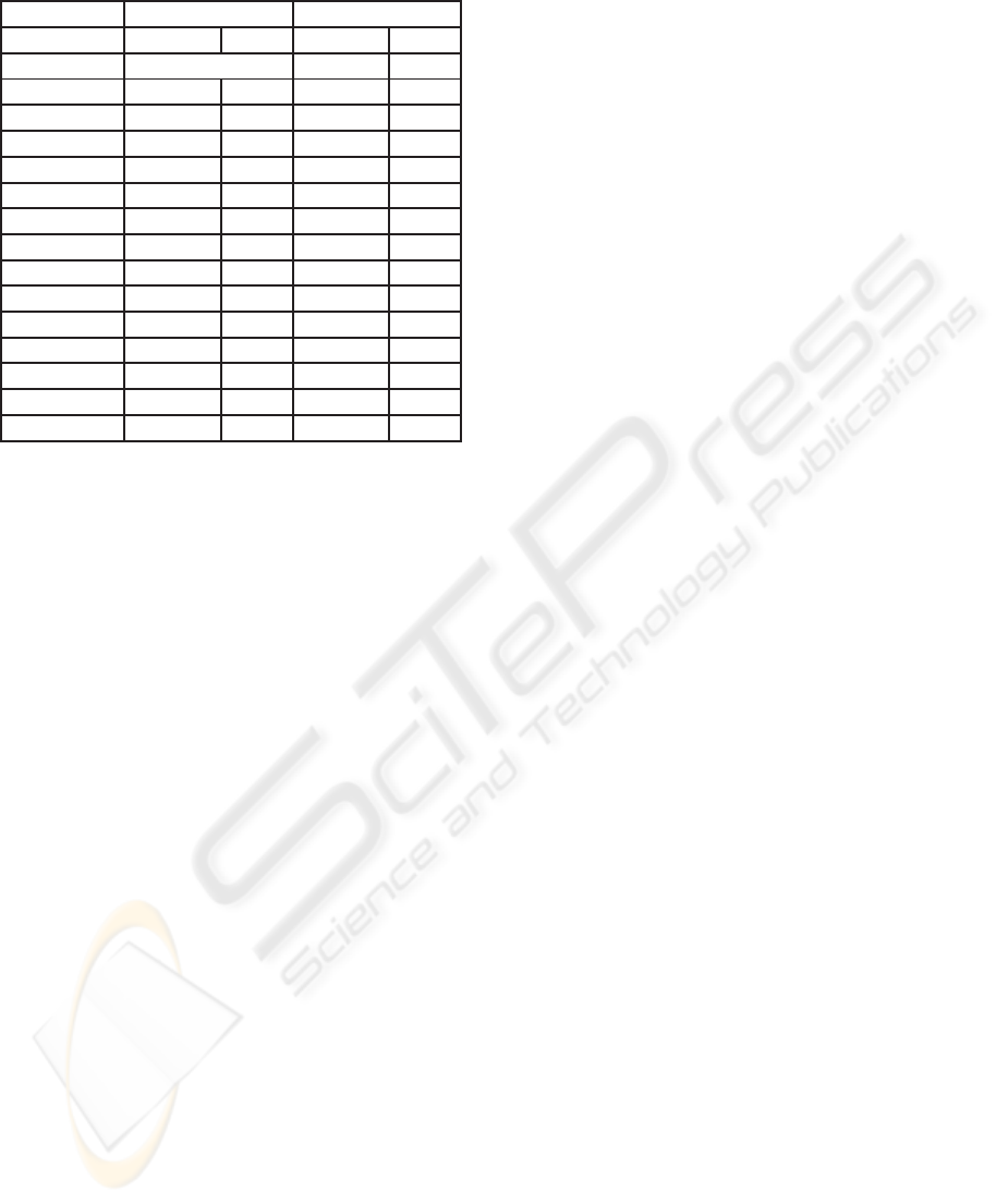
Table 3: Experimental Results: III.
Recursive Rec-Backward
Example time splits time splits
1-flow unknown 0.32 1
2-tanks 0.26 3 0.28 1
car 1.29 0 1.07 0
circuit 53.12 171 68.28 192
clock 1.97 16 0.74 14
convoi-1 2.70 0 1.71 0
convoi 2177.75 374 1830.56 300
eco 253.19 290 5.77 22
focus 2.79 48 0.42 8
mixing 104.96 109 1.75 0
mutant 1978.43 195 1850.17 191
real-eigen 0.59 2 0.61 0
s-focus 0.53 2 0.44 1
trivial-hard 0.07 4 0.05 0
VDP 25.81 64 0.77 1
splitting steps. The reason is that although the com-
bined version is more successful in pruning, the split-
ting heuristics will sometimes choose different boxes
which then results—in rare cases—in more necessary
splits. (2) For all examples except one, the recursive
version needs less splitting steps than the forward ver-
sion. However, for the eco example, the recursive
version needs more splitting steps. This is due to the
same reason as above—moresuccessful pruning leads
to different box choices. Again, for some example the
CPU time is worse since the constraints in the recur-
sive version are more complex. (3) Again with one
exception (circuit), the combined recursive and back-
ward version always needs less splitting steps than
both the recursive version and combined forward and
backward version, often even much less. For most ex-
amples also the run-time improved, sometimes over
an order of magnitute. Only for two additional, rather
easy examples (car, convoi-1), the CPU time slightly
increases since the constraints in the combined recur-
sive and backward version are more complex.
Summarizing, the contributions of this paper re-
sult in a definite and robust efficiency improvement
of the algorithms.
8 CONCLUSIONS
In this paper we have introduced two improvements
to a method of safety verification of hybrid sys-
tems by constraint propagation based abstraction re-
finement. The provided computational experiments
clearly show the advantage of proposed improve-
ments. We will base future improvements of the
method on a detailed study of the behavior of the used
algorithms on further benchmark problems.
ACKNOWLEDGEMENTS
The work of the first author has been supported by
GA
ˇ
CR grant 201/08/J020 and by the institutional re-
search plan AV0Z100300504. The second author was
partly supported by the National Key Basic Research
Program of China under Grant No. 2005CB321902
and the Program for Excellent Talents of Beijing un-
der Grant No. 20071D1600600410.
REFERENCES
Benhamou, F. and Granvilliers, L. (2006). Continuous and
interval constraints. In Rossi, F., van Beek, P., and
Walsh, T., editors, Handbook of Constraint Program-
ming, pages 571–603. Elsevier Amsterdam.
Frehse, G., Krogh, B. H., and Rutenbar, R. A.
(2006). Verifying analog oscillator circuits using
forward/backward abstraction refinement. In DATE
2006: Design, Automation and Test in Europe.
Kloetzer, M. and Belta, C. (2006). Reachability analysis of
multi-affine systems. In Hespanha, J. and Tiwari, A.,
editors, HSCC’06, volume 3927 of LNCS. Springer.
Preußig, J., Stursberg, O., and Kowalewski, S. (1999).
Reachability analysis of a class of switched contin-
uous systems by integrating rectangular approxima-
tion and rectangular analysis. In Vaandrager, F. and
van Schuppen, J., editors, HSCC’99, number 1569 in
LNCS. Springer.
Ratschan, S. and She, Z. (2004). HSOLVER.
http://hsolver.sourceforge.net. Software package.
Ratschan, S. and She, Z. (2006). Constraints for continuous
reachability in the verification of hybrid systems. In
Proc. AISC’2006, number 4120 in LNCS. Springer.
Ratschan, S. and She, Z. (2007). Safety verification of
hybrid systems by constraint propagation based ab-
straction refinement. ACM Transactions on Embedded
Computing Systems, 6(1).
RECURSIVE AND BACKWARD REASONING IN THE VERIFICATION ON HYBRID SYSTEMS
71
