
THE APPLICATION OF REFERENCE-PATH CONTROL TO
VEHICLE PLATOONS
Drago Matko, Gregor Klanˇcar, Saˇso Blaˇziˇc
Faculty of electrical engineering University of Ljubljana, Slovenia
Olivier Simonin
lab: LORIA Maia project, University of Henri Poincare, Nancy, France
Franck Gechter, Jean-Michel Contet, Pablo Gruer
Systems and Transportation Laboratory (SET), University of Technology of Belfort-Montb´eliard (UTBM), Belfort, France
Keywords:
Platoon, reactive multiagent, longitudinal and lateral control, reference-path following control.
Abstract:
A new algorithm for the control of vehicle platooning is proposed and tested on a robot-soccer test bed. We
considered decentralized platooning, i.e., a virtual train of vehicles, where each vehicle is autonomous and
decides on its motion based on its own perceptions. The platooning vehicles have non-holonomic constraints.
The following vehicle only has information about its own orientation and about its distance and azimuth to
the leading vehicle. Its position is determined using odometry and a compass. The reference position and the
orientation of the following vehicle are determined by the estimated path of the leading vehicle in a parametric
polynominal form. The parameters of the polynominals are determined using the least-squares method. This
parametric reference path is also used to determine the feed-forward part of the applied control algorithm.
The feed-back control consists of a state controller with three inputs: the longitudinal and lateral position
errors and the orientation error. The results of the experiments demonstrate the applicability of the proposed
algorithm for vehicle platoons.
1 INTRODUCTION
Vehicle platoon systems are a promising approach
for new transportation systems because of their inno-
vative capabilities. Their main goals, when applied
to passenger cars are (i) an increase in the vehicle
density on the highway (i.e., avoiding traffic jams),
and (ii) security improvements thanks to automated
or semi-automated driving assistance (adaptive cruise
control, obstacle detection and avoidance, automatic
car parking, etc.). Most of these platooning systems
are based on a linear configuration (i.e., a virtual train
of vehicles).
Among the several problems associated with the
control of platooning systems, longitudinal and lateral
control are the most important.
Longitudinal control involves controlling the
braking and acceleration in order to stabilize the dis-
tance between the leading vehicle and the follow-
ing vehicle. This control takes as a parameter the
distance between the leading and the following ve-
hicles. Sheikholeslam and Desoer (Sheikholeslam
and Desoer, 1993) proposed a form of longitudi-
nal control based on linearization methods. Ioan-
nou and Xu (Ioannou and Xu, 1994) controlled the
brakes and the acceleration using a fixed-gain PID
control with gain scheduling. In contrast, Hedrick,
Tomizuka and Varaiya (Hedrick et al., 1994) used a
control mode based on a non-linear method with PID.
Lee, Tomizuka, Jung and Kim (Lee and Tomizuka,
2003; Lee et al., 2000) proposed a longitudinal con-
trol based on fuzzy logic.
Lateral control involves aligning the vehicle’s di-
rection relative to the vehicle in front. Daviet and
Parent (Daviet and M.Parent, 1996) proposed a form
of lateral control using a PID controller. This con-
trol consists of keeping the angle between the lead-
ing and the following vehicles close to zero. In
the literature, papers can be found dealing with lat-
eral and longitudinal control using physics-inspired
models. For instance, Gehrig and Stein (Gehrig and
Stein, 2001) designed a model based on particles’
145
Matko D., Klanc
ˇ
ar G., Blaži
ˇ
c S., Simonin O., Gechter F., Contet J. and Gruer P. (2008).
THE APPLICATION OF REFERENCE-PATH CONTROL TO VEHICLE PLATOONS.
In Proceedings of the Fifth International Conference on Informatics in Control, Automation and Robotics - RA, pages 145-150
DOI: 10.5220/0001476801450150
Copyright
c
SciTePress
submissive forces, whereas Yi and Chong (Yi and
Chong, 2005) developedan impedance-controlimma-
terial hook model. Halle and Chaib-draa (Halle and
Chaib-draa, 2005) used a Multi-Agent System (MAS)
in order to model immaterial vehicles using constant
values from (Daviet and M.Parent, 1996). Contet,
Gechter, Gruer and Koukam (Contet et al., 2007) pro-
posed a solution for longitudinal and lateral control
using Newtonian forces in an interactive model. In
Bom et. all (Bom et al., 2005) a global platooning
control strategy is proposed using nonlinear control
law which decouples lateral and longitudinal control.
In this paper a novel approach to a platoon of non-
holonomic vehicles using the well-known state-space
control of nonholonomic systems is presented. The
vehicle platooning control strategy relays on relative
information to preceding vehicles only therefore no
explicit inter-vehicle data exchange and global global
information (such as GPS) is required. The impor-
tant advantage here is that relative information can
be measured with low cost sensor sets. Additionally
the method to obtain on-line objectives for the fol-
lower vehicles control is presented, where the inter-
vehicle distance is curvilinear one as also proposed in
(Bom et al., 2005). The proposed control algorithm
was tested in simulations and on a platoon of soccer
robots.
Controlling nonholonomic systems as they follow
a reference path is a well-known problem that has
been studied by many authors (Kolmanovskyand Mc-
Clamroch, 1995; Luca and Oriolo, 1995; Sarkar et al.,
1994). The control of vehicles, especially mobile
robots, by considering only the first-order kinematics
is very common in the literature ((Canudas de Wit and
Sordalen, 1992; Oriolo et al., 2002; Balluchi et al.,
1996)) as well as in practice. The vehicle has to con-
sider nonholonomic constraints, so its path cannot be
arbitrary. Moreover in an environment with obstacles,
limitations and other demands the vehicle should be
controlled on a reference path, which should follow
all the kinematic constraints and avoids obstacles.
The paper is organized as follows: In Section 2 a
model of nonholonomic systems and the correspond-
ing control law that can be applied to such systems
are presented. The application of the proposed con-
trol law to platoon systems is derived in Section 3.
The results of the tests on a robot-soccer set-up are
presented in Section 4.
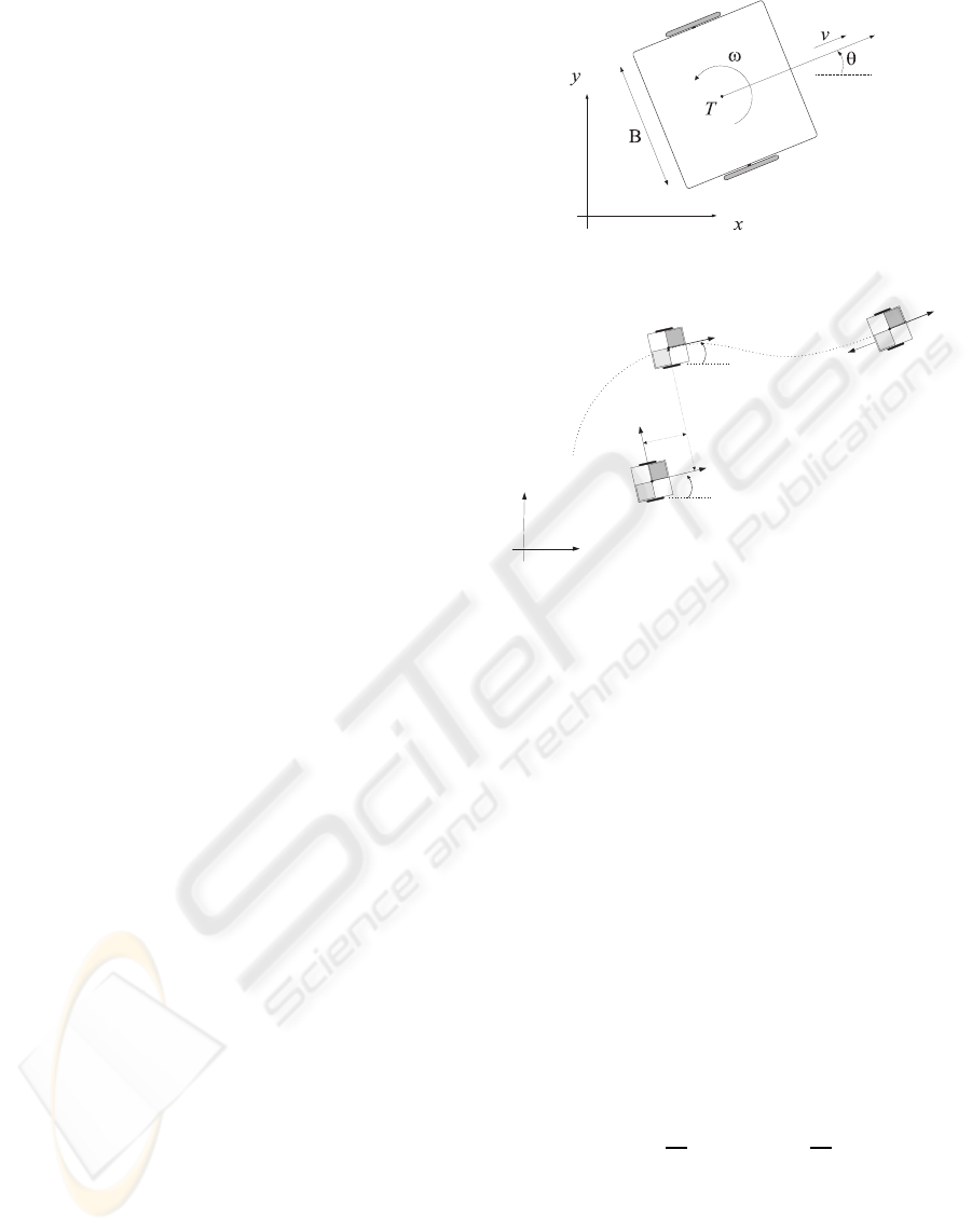
Figure 1: Vehicle architecture and symbols.
referencevehicle
leading
vehicle
followingvehicle
q
r
q
( , )x y
r r
( , )xy
x
y
x
y
e
1
e
2
t
L
Figure 2: Illustration of the error transformation.
2 MODELING AND CONTROL
OF NONHOLONOMIC
SYSTEMS
In the following the direct and inverse kinematics for
mobile vehicles with a differential drive are deter-
mined. The vehicle’s architecture, together with its
symbols, is shown in the Fig. 1, where it is supposed
that the geometrical centre T and the centre of gravity
coincide.
The equations of motion are as follows
˙x
˙y
˙
θ
=
cosθ 0
sinθ 0
0 1
·
v
ω
(1)
where v and ω are the tangential and angular veloc-
ities of the platform shown in the Fig. 1. The right
and left velocities of the vehicle’s wheels are then ex-
pressed as v
R
= v+
ωB
2
and v
L
= v−
ωB
2
, respectively,
where B is the distance between the robot wheels.
For a given reference trajectory (x
r
(t), y
r
(t)) de-
fined in the time interval t ∈[0,T] the feed-forward
control law can be derived. From the obtained inverse
kinematics the vehicle inputs are calculated, these
drive the vehicle on the desired path only if there are
no disturbances and no initial state errors. The re-
quired vehicle inputs, the tangential velocity v
f f
and
ICINCO 2008 - International Conference on Informatics in Control, Automation and Robotics
146
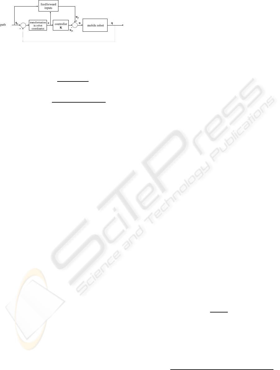
Figure 3: Mobile-vehicle control schematic.
the angular velocity ω
f f
, are calculated from the ref-
erence path. The tangential velocity is given by
v
f f
(t) =
q
˙x
2
r
(t) + ˙y
2
r
(t) (2)
ω
f f
(t) =
˙x
r
(t) ¨y
r
(t) − ˙y
r
(t) ¨x
r
(t)
˙x
2
r
(t) + ˙y
2
r
(t)
(3)
When a vehicle is controlled to drive on a refer-
ence path, it usually has some following error. This
following error, expressed in terms of the real vehi-
cle, as shown in the Fig. 2, is given by
e
1
e
2
e
3
=
cosθ sinθ 0
− sinθ cosθ 0
0 0 1
·
x
r
− x
y
r
− y
θ
r
− θ
(4)
In the Fig. 2 the reference vehicle is an imaginary
vehicle that ideally follows the reference path. In con-
trast, the real vehicle (when compared to the reference
vehicle) has some error when following the reference
path. Therefore, the control algorithm was designed
to force the vehicle to follow the reference path pre-
cisely as proposed in (Luca and Oriolo, 1995; Oriolo
et al., 2002). It is as follows
v
r
= v
f f
cose
3
− v
fb
ω
r
= ω
f f
− ω
fb
(5)
where v
r
and ω
r
are reference velocities (set-points)
for the low level control controlling the wheels of the
vehicle and v
fb
, ω
fb
are the outputs of the feed-back
controller given by
v
fb
ω
fb
=
−k
1
0 0
0 −sign(u
f f
)k
2
−k
3
·
e
1
e
2
e
3
(6)
The schematic of the obtained control is explained
in Fig. 3. The gains k
1
, k
2
and k
3
of the state feed-
back controller K were determined by trial and error.
3 APPLICATION OF THE
CONTROLLER TO A LINEAR
PLATOON
It is supposed that there is no data communication be-
tween the leading and following vehicles. The fol-
lowing vehicle measures the distance and the azimuth
(relative to its own orientation)) of the leading vehi-
cle. To ensure stable control also a measurement of
the orientation of the following vehicle (e.g. with a
compass) is also needed. No other sensors (e.g., GPS)
are required. All the positions are treated in a coordi-
nate system that is fixed to the ground. The following
vehicle determines its own position using odometry.
Having the current position X(k) = [x(k),y(k)]
T
, the
position in the next sample is determined by a simple
Euler integration
X(k+ 1) = X(k) +
cos(θ)
sin(θ)
v
ref
∆t (7)
where θ is the orientation of the following vehicle,
v
ref
is the reference speed of the vehicle and ∆t is the
sample time. As shown later, the method of integra-
tion and the associated errors in the accuracy of the
absolute position are not significant, since only the
relative position of both vehicles is important.
The path of the leading vehicle X
h
(k) =
[x
h
(k)y
h
(k)]
T
is calculated by the following vehicle
using its current position and the measurements of the
distance D and the azimuth θ
a
(e. g., by using a laser
range finder) as follows:
X
h
(k) = X(k) +
cos(θ+ θ
a
)
sin(θ+ θ
a
)
D (8)
This information is stored in the memory and repre-
sented in parametric form (with the parameter k - re-
lated in the time t = k∆t). The following vehicle is
supposed to track the leading vehicle at a distance L
- measured on the path of the leading vehicle. First,
the time T needed by the leading vehicle to drive the
distance L is calculated using
L =
Z
T
0
q
˙x
2
h
+ ˙y
2
h
dt (9)
This time T is calculated by a linear interpolation
of the two successive time instants (k+1 and k) defin-
ing the time internal where the numerically calculated
distance L
′
becomes greater than the desired distance
L.
L
′
=
N
∑
k=0
q
[x
h
(k+ 1) − x
h
(k)]
2
+ [y
h
(k+ 1) − y
h
(k)]
2
(10)
THE APPLICATION OF REFERENCE-PATH CONTROL TO VEHICLE PLATOONS
147
According to relation (4) the interpolated value for
time T is obtained by T = k∆t +
∆t
L
′
(k+1)−L
′
(k)
(L −
L
′
(k)), where L is the desired tracking distance among
the vehicles. Next, the path shape of the leading ve-
hicle at the moment −T (T seconds in the past) is
expressed in the parametric polynomial form
x
h
(t) = a
x
2
t
2
+ a
x
1
t + a
x
0
(11)
y
h
(t) = a
y
2
t
2
+ a
y
1
t + a
y
0
(12)
The coefficients of the polynomials a
x
i
and a
y
i
are
calculated using the least-squares method with more
than three samples around the time T (seven were
used in our experiments). The reference position
and the orientation of the following vehicle are de-
termined using
X
r
=
x
h
(T)
y
h
(T)
=
a
x
2
T
2
+ a
x
1
T + a
x
0
a
y
2
T
2
+ a
y
1
T + a
y
0
(13)
θ
r
= arctg
2a
y
2
T + a
y
1
2a
x
2
T + a
x
1
(14)
respectively. In the Fig. 2 they are denoted as the ref-
erence vehicle. The tangential and angular velocities
of the reference vehicle (needed for the feed-forward
control) are
v
r
(t) =
q
(2a
x
2
T + a
x
1
)
2
+ (2a
y
2
T + a
y
1
)
2
(15)
and
ω
r
(t) =
(2a
x
2
T + a
x
1
) × 2a
y
2
− (2a
y
2
T + a
y
1
) × 2a
x
2
(2a
x
2
T + a
x
1
)
2
+ (2a
y
2
T + a
y
1
)
2
(16)
respectively. For the feed-back control the error vec-
tor is given according to Eq. (4) by
e =
cosθ sinθ 0
− sinθ cosθ 0
0 0 1
X
r
− X
θ
r
− θ
(17)
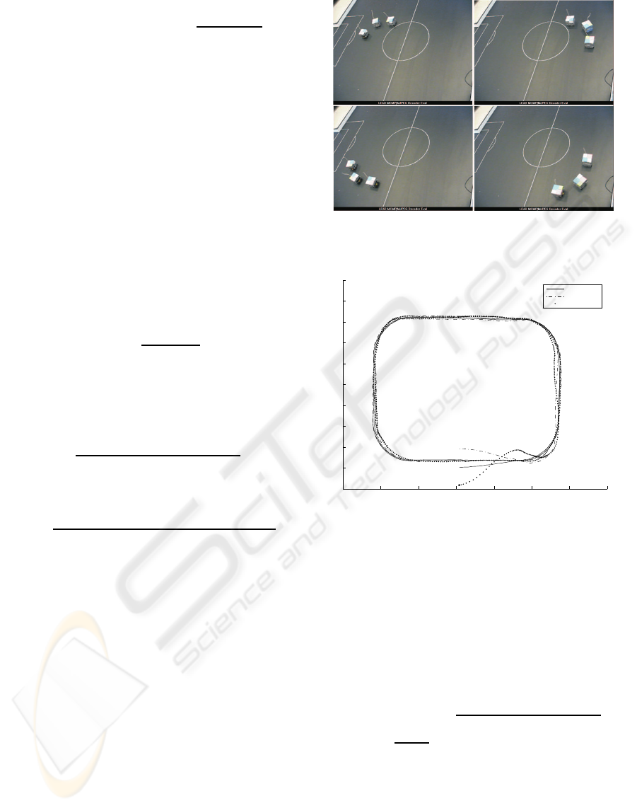
4 RESULTS OF THE
EXPERIMENTS
The proposed algorithm was tested on a robot-soccer
set-up (see Fig. 4) consisting of three Middle League
MiroSot category robots of size 7.5 cm cubed, a dig-
ital color camera and a personal computer. The color
camera mounted above the pitch is a global sensor.
The vision part of the programme ((Klanˇcar et al.,
2004)) processes the incoming image to identify the
positions and orientations of the robots. The first,
(leading) robot was driven on a prescribed path. The
Figure 4: Real set-up experiment.
0.4 0.6 0.8 1 1.2 1.4 1.6 1.8
0.4
0.5
0.6
0.7
0.8
0.9
1
1.1
1.2
1.3
Three real mobile robots platoon
first robot
second robot
third robot
Figure 5: Results of real experiments.
second (the first following) robot receives only the in-
formation about its distance and azimuth to the first
robot and its own orientation. The third (the sec-
ond following) robot receives only the information
about its distance and azimuth to the second robot
and its own orientation. The noisy position esti-
mates of the used camera sensor influences the cal-
culated distance and azimuth information. The esti-
mated noise deviation of measured robots positions
was ±5mm. The distances and azimuth orientations
are obtained by D
i
=
p
(x
i−1
− x
i
)
2
+ (y
i−1
− y
i
)
2
and
θ
ai
= arctan
y
i−1
−y
i
x
i−1
−x
i
, where i = 2,3 is robot index.
The parameters values of the controller (5) were
k
1
= 2,k
2
= 20, k
3
= 2, sampling time was ∆t = 33ms
and the desired tracking distance was L = 20cm. The
results of the tests are shown in the Fig. 5. The film
of the real experiment can be seen at (Klanˇcar, 2008).
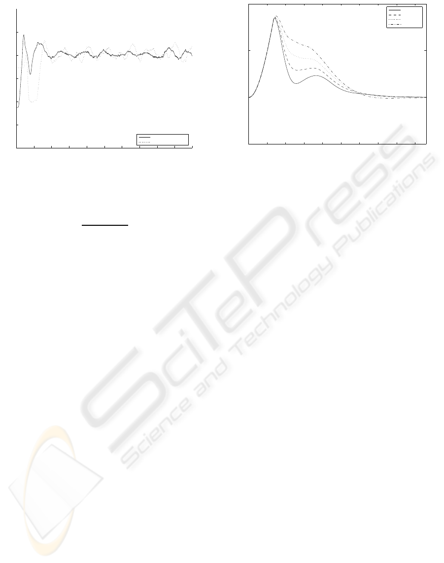
In the Fig. 6 the time course of the distance be-
tween the robots is presented . The distance was
calculated with assumption that the path between the
ICINCO 2008 - International Conference on Informatics in Control, Automation and Robotics
148
0 2 4 6 8 10 12 14 16 18 20
0
0.05
0.1
0.15
0.2
0.25
Time [s]
Distance [m]
Distance of robots − Real
first to second robot
second to third robot
Figure 6: Distance between robots - experiment.
robots is an arc, which results in
L
arch
=
∆θ
2sin(∆θ/2)
× D (18)
where D is the straight line between the robots and ∆θ
is the difference in their orientation angles. It is clear
that after a transition phase (the merging and splitting
of the platoons is currently under investigation) the
second and third vehicle follow with acceptable accu-
racy. The results of the real experiments are slightly
worse due to the noise in the position estimation and
due to the time delay of the optical tracking and recog-
nition. The accuracyof the integration method and the
associated error, which is equivalent to the slipping of
the vehicle’s wheels, is analysed and illustrated in the
Fig. 7, where the distance between the leading and
the following platoon robots in a straight path is illus-
trated. It can be seen that the constant slipping of the
wheels has no influence on the steady-state distance
of the platoon vehicles. This conclusion makes sense
since servoing accuracy should not be destroyed be-
cause relative information among vehicles (distances
and azimuth orientations) are always obtained from
accurate relative sensor.
5 CONCLUSIONS
A new algorithm for the control of vehicle platoons
was proposed. The following vehicle only has infor-
mation about its own orientation and about the dis-
tance and azimuth of the leading vehicle. Its own po-
sition is determined using odometry and a compass. It
calculates the reference path in a parametric polyno-
mial form, and the parameters of the polynomials are
determined by the least-squares method. Having the
reference path, the feed-forward and feed-back con-
0 0.5 1 1.5 2 2.5 3 3.5 4 4.5
0.15
0.2
0.25
Time [s]
Distance [m]
Slip = 0%
Slip = 10%
Slip = 20%
Slip = 30%
Figure 7: Distance between robots with slip in a straight
path (simulation).
trol are applied to the following vehicle. The fol-
lowing vehicle calculates its own position by means
of a simple Euler integration. It was established that
the error in the integration procedure (equivalent to
the errors due the wheel slipping) has a minor influ-
ence on the accuracy of the platoon distance. The pro-
posed algorithm was tested on a robot-soccer test bed.
The results confirm the applicability of the proposed
method.
REFERENCES
Balluchi, A., Bicchi, A., Balestrino, A., and Casalino, G.
(1996). Tracking control for dubin’s cars. In Pro-
ceedings of the 1996 IEEE International Conference
on Robotics and Automation,Minneapolis, Minnesota,
pp. 3123-3128.
Bom, J., Thuilot, B., Marmoiton, F., and Martinet, P.
(2005). A global control strategy for urban vehicles
platooning. relying on nonlinear decoupling laws. In
Proceedings of the 2005 IEEE/RSJ International Con-
ference on Intelligent Robots and Systems, Alberta,
pp. 1995-2000,.
Canudas de Wit, C. and Sordalen, O. J. (1992). Exponen-
tial stabilization of mobile robots with nonholonomic
constraints. In IEEE Transactions on Automatic Con-
trol, Vol. 37, No. 11, pp. 1791-1797.
Contet, J., Gechter, F., Gruer, P., and Koukam, A. (2007).
Application of reactive multiagent system to linear
vehicle platoon. In Annual IEEE International Con-
ference on Tools with Artificial Intelligence(*ICTAI*),
Grece, Patras.
Daviet, P. and M.Parent (1996). Longitudinal and lateral
servoing of vehicles in a pltoon. In IEEE Intelligent
Vehicles Symposium, Proceedings, pages 41-46,.
Gehrig, S. K. and Stein, F. (2001). Elastic bands to en-
hance vehicle following. In IEEE Conference on In-
THE APPLICATION OF REFERENCE-PATH CONTROL TO VEHICLE PLATOONS
149

telligent Transportation Systems, Proceedings, ITSC,
pages 597-602.
Halle, S. and Chaib-draa, B. (2005). A collaborative driv-
ing system based on multiagent modeling and simula-
tions. In Transp. Res. C, Emerg. Technol. (UK), 13(4):
320 - 45.
Hedrick, J., Tomizuka, M., and Varaiya, P. (1994). Control
issues in automated highway systems. In IEEE Con-
trol Systems Magazine, 14(6):21-32.
Ioannou, P. and Xu, Z. (1994). Throttle and brake con-
trol systems for automatic vehicle following. In IVHS
Journal,1(4):345.
Klanˇcar, G. (2008). http://msc.fe.uni-lj.si/publicwww
/klancar/robotsplatoon.html.
Klanˇcar, G., Kristan, M., and S. Kovaˇciˇc, O. O. (2004). Ro-
bust and efficient vision system for group of cooper-
ating mobile robots with application to soccer robots.
In ISA Transactions, vol. 43, pp. 329-342.
Kolmanovsky, I. and McClamroch, N. H. (1995). Devel-
opments in nonholonomic control problems. In IEEE
Control Systems, Vol. 15, No. 6, pp. 20-36.
Lee, H. and Tomizuka, M. (2003). Adaptive vehicle traction
force control for intelligent vehicle highway systems
(ivhss). In IEEE Transactions on Industrial Electron-
ics, 50(1):37-47.
Lee, M., Jung, M., and Kim, J. (2000). Evolutionary
programming-based fuzzy logic path planner and fol-
lower for mobile robots. In Proceedings of the IEEE
Conference on Evolutionary Computation, ICEC, (1)
pp 139-144.
Luca, A. and Oriolo, G. (1995). Modelling and control
of nonholonomic mechanical systems. In Kinemat-
ics and Dynamics of Multi-Body Systems,Springer-
Verlag, Wien.
Oriolo, G., Luca, A., and Vandittelli, M. (2002). Wmr con-
trol via dynamic feed-back linearization: Design, im-
plementation, and experimental validation. In IEEE
Transactions on Control Systems Technology, Vol. 10,
No. 6, pp. 835-852.
Sarkar, N., Yun, X., and Kumar, V. (1994). Control of me-
chanical systems with rolling constraints: Application
to dynamic control of mobile robot. In The Interna-
tional Journal of Robotic Research, Vol. 13, No. 1, pp.
55-69.
Sheikholeslam, S. and Desoer, C. (1993). Longitudinal
control of a platoon of vehicles with no communi-
cation of lead vehicle information: A system level
study. In IEEE Transactions on Vehicular Technology,
42(4):546-554.
Yi, S.-Y. and Chong, K.-T. (2005). Impedance control
for a vehicle platoon system. In Mechatronics (UK),
15(5):627-38.
ICINCO 2008 - International Conference on Informatics in Control, Automation and Robotics
150
