A NEW APPROACH OF GRAY IMAGES BINARIZATION FOR

ARTIFICIAL VISION SYSTEMS WITH THRESHOLD METHODS

Andrei Hossu and Daniela Hossu

University Politehnica of Bucharest, Faculty of Control and Computers

Dept. of Automatics and Industrial Informatics, 313 Spl. Independentei, sector 6, RO-77206, Bucharest, Romania

Keywords: Vision systems, Gray level image binarization, gray level histogram, global optimum thresholding, dynamic

optimum threshold, temporal histogram, temporal thresholding and moving scene in robotic automation.

Abstract: This paper presents some aspects of the (gray level) image binarization methods used in artificial vision

systems. It is introduced a new approach of gray level image binarization for artificial vision systems

dedicated to the specific class of applications for moving scene in industrial automation – temporal

thresholding. In the first part of the paper are remarked some limitations of using the global optimum

thresholding in gray level image binarization. In the second part of this paper are presented some aspects of

the dynamic optimum thresholding method for gray level image binarization. In the third section are

introduced the concepts of temporal histogram and temporal thresholding, starting from classic methods of

global and dynamic optimal thresholding of the gray level images. In the final part are presented some

practical aspects of the temporal thresholding method in artificial vision applications for the moving scene

in robotic automation class; highlighting the influence of the acquisition frequency on the methods results.

1 IMAGE BINARIZATION WITH

GLOBAL THRESHOLD

Threshold methods are defined as starting from the

analyse of the values of a function T of the type:

T = T [x, y, p(x, y), f(x, y)] (1)

Where:

f(x, y) – represents the intensity value of the

image element located on the co-ordinates (x, y);

p(x,y) – represents the local properties of the

specific point (like the average intensity of a region

centred in the co-ordinates (x, y)).

T – is the binarization threshold

The goal is to obtain from an original gray level

image, a binary image g(x, y) defined by:

⎩

⎨

⎧

≤

Tyxf

yxg

),(for 0

),(for 1

),(

(2)

For T a function only of f(x, y), the obtained

threshold is called global threshold.

In the case of T a function of both f(x, y) and p(x,

y), the obtained threshold is named local threshold.

In the case of T a function of all f(x, y), p(x, y), x

and y, the threshold is a dynamic threshold.

1.1 Intensity Level on Normal

Distribution Assumption

Gray level histogram represents the probability

density function of the intensity values of the image.

In order to simplify the explanations, we suppose

the image histogram of the gray levels is composed

from two values combined with additive Gaussian

noise:

- The first segment of the image histogram

corresponds to the background points – the intensity

levels are closer to the lower limit of the range (the

background is dark)

- The second segment of the image histogram

corresponds to the object points – the intensity levels

are closer to the upper limit of the intensity range

(the objects are bright).

The problem is to estimate a value of the

threshold T for which the image elements with an

intensity value lower than T will contain background

points and the pixels with the intensity value greater

than T will contain object points, with a minimum

error. For a real image, the partitioning between the

Hossu A. and Hossu D. (2008).

A NEW APPROACH OF GRAY IMAGES BINARIZATION FOR ARTIFICIAL VISION SYSTEMS WITH THRESHOLD METHODS.

In Proceedings of the Fifth International Conference on Informatics in Control, Automation and Robotics - RA, pages 11-16

DOI: 10.5220/0001477200110016

 SciTePress

two brightness levels is not so simple and also not so

accurate. The partitioning is fully accurate only if

the two modes of the bimodal histogram are not

overlapped. The classification is defined as the

process of the distribution of the pixels in classes.

The goal of the binarization process is the

minimisation of the error of classification. The

optimum binarization threshold is located in the

intersection position of the two normal distributions.

The estimation of the error of classification is

obtained from the area of the overlapped segments:

image size

(3)

Suppose the image contains two intensity level

values affected with additive Gaussian noise. The

mixture probability density function is:

)()()(

2211

xpPxpPxp

(4)

Where:

x – the random value representing the intensity

level,

(x), p

(x) – are the probability density

functions,

, Pp

- are the a priori probabilities of the two

intensity levels (P

= 1).

For the normal distribution case on the two

brightness levels:

)(

exp

)(

exp

)(

μ−

πσ

μ−

πσ

xPxP

(5)

Where:

)()()(

2211

xpPxpPxp

(6)

, μμ - are the mean values of the two

brightness levels (the two modes),

, σσ - are the standard deviations of the two

statistical populations.

Suppose the background is darker than the

object. In this case

μ<μ and defining a threshold

T, so that all pixels with intensity level below T are

considered belonging to the background and all

pixels with level above T are considered object

points. The probability of misclassification an object

point (classifying an object point as a background

point) is:

Similarly, E

dxxpTE

)()(

∫

∞+

∞−

(7)

The probability of error is given by:

)()()(

1221

TEPTEPTE

(8)

To find the threshold value for which the error is

minimum, E(T) is differentiate with respect to T:

tpPtpP ()(

2211

)

(9)

Applying the result to the Gaussian density we

obtain:

+ BT + C = 0 (10)

Where:

)(2

σσ+μσ−μσ=

σμ−σμ=

σ−σ=

(11)

If the standard deviations are equal, a single

threshold is sufficient:

2 p

μ−μ

μ+μ

(12)

If the probabilities are equal p

= p

the threshold

value is equal with the average of the means.

A way of checking the validity of the assumption

of bimodal histogram is to estimate the mean-square

error between the mixture density, p(x) and the

experimental histogram h(x

)]()([

xhxp

M −=

∑

(13)

Where: N – number of possible levels of the

image (usually N = 256)

The image binarization is obtained changing the

colour attribute of each pixel according to its

intensity level relative to the binarization threshold.

Characteristics of the global thresholding methods

(Borangiu, et al., 1994)., (

Haralick and Shapiro, 1992):

- The assumption that both classes have the same

standard deviation is acceptable, but the assumption

the classes (two levels) have the same a priori

probabilities in many applications is not acceptable.

In the case of the artificial vision systems

dedicated to object recognition for industrial

applications there is a large amount of a priori

information about the image that has to be

processed. Better results of estimation of the

distribution of the image elements of the scene

(background image, without the objects) can be

obtained. Usually, in robotic applications, the

illumination environment is known and controlled

ICINCO 2008 - International Conference on Informatics in Control, Automation and Robotics

and also the object classes with a probability of

apparition in the image are not known. In many

robotic application an estimation of the ratio

between the area of the objects to be analysed and

the total area of the image scene, can be made with

good results (a batter estimation than the assumption

of P

= P

= 0.5).

2 IMAGE BINARIZATION WITH

DYNAMIC THRESHOLD

There are some classes of scenes of artificial vision

systems where using the global threshold methods is

not acceptable:

• The case of the applications where the lighting

system does not supply a uniform intensity all over

the analysed surface.

• Segments of the image (or some times, image

elements) do not have the same behaviour in the

same lighting conditions.

For these types of images, for binarization of the

image, the most often used are dynamic threshold

methods. The methods are based on the local analyse

of the image. The algorithm of the estimation of the

dynamic threshold consist of:

• The original image is divided in regions of a

prescribed size.

• For each region it is estimated the histogram

• For each histogram it is estimated the error

induced from the assumption of bimodal histogram

(a histogram built from two normal distributions)

• If the value of the error is less than an

acceptable value, the global threshold for the region

is estimated.

• If the value of the error is too big (the

histogram is too far from a bimodal histogram) the

threshold value for binarization is estimated from the

interpolation of the neighbours region threshold

values (for which the assumption of a bimodal

histogram is considered acceptable).

• In the final stage, a second interpolation process

is applied: for each image element is assigned a

threshold value T(x, y) from the interpolation of the

values of the neighbour image elements.

The method is called dynamic thresholding

because the value of the resulted threshold for each

image element is dependent of the position of the

element in the image - T(x, y).

Characteristics of the dynamic thresholding

methods:

- Lack of processing time consumption – each

element of the image is used at least two times (the

method requires multiple-pass of the image) in

different steps of the algorithm (and the number of

the elements is very large).

- Estimation of the acceptable error value (or the

validation of the bimodal histogram assumption) is a

complex process.

- To choose the size of the image regions we

have to take into account:

- Large size of the region makes the method to

loose the dynamic threshold characteristics and to

fail into a global threshold method

- Small size of the region makes to loose the

statistical characteristic of the population of the

image elements contained by the analysed region

(and the accuracy of the results is lost).

The last comment on the method is the fact that

this method does not solve the problem of the non-

uniformity of the illumination system or of the

acquisition sensor.

3 TEMPORAL HISTOGRAM

For the class of artificial vision systems dedicated

for moving scene (used very often in inspection and

robotic applications) three types of image intensity

level distortions can be identified (Croicu, et al.,

1998), (Hossu, et al., 1998):

• Illumination non-uniformity (obtaining a

uniform intensity of the light on the whole area of

the scene where the image is analysed – usually 2 m

– it is practical impossible).

• Sensor non-linearity – for linear cameras with a

large number of pixels per row (2048 and more) can

be identified areas of non-linear behaviour of the

sensor (there are segments of the linear sensor with a

different behaviour of the elements sensitivity at

light intensity).

• Sensor cells non-uniformity – in cameras with

CCD sensor, the cells presents a different response

on sensitivity at light intensity related to their

neighbours

In Figure 1 are presented the image intensity

level distortions.

The main problem of the methods presented before

represents the assumption that the image is a

statistical population obtained from the addition of

two ore more distributions (in the general accepted

case normal distribution).

A NEW APPROACH OF GRAY IMAGES BINARIZATION FOR ARTIFICIAL VISION SYSTEMS WITH

THRESHOLD METHODS

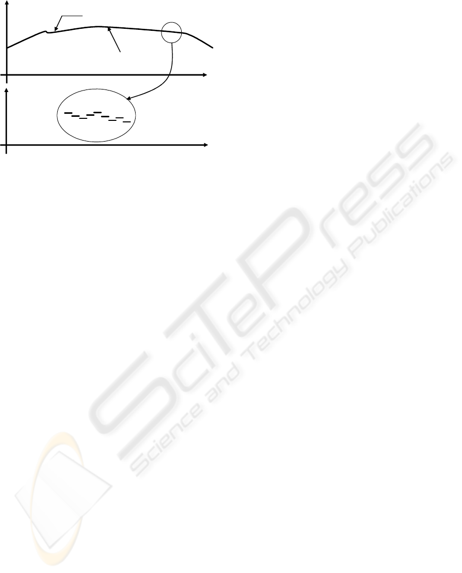
Pixel value

Sensor non-linearity

Illumination non-

uniformity

Cell non-uniformity

Pixels row

Figure 1: Image intensity level distortions for CCD linear

camera acquisition.

In the general case (an array image) an image

represents a data set of:

{f(x, y) | x ∈ [0,N], y ∈ [0,M]}

(14)

where:

N represents the number of image elements per

row (number of image columns),

M represents the number of image elements per

column (number of image rows),

In the linear image case, this data set become:

{f(x) | x ∈ [0,N]}

(15)

where:

N represents the number of image elements per

row (number of image columns).

This assumption on the distribution of the

intensity levels has the starting point the assumption

that the insertion point of the noise is located on the

transmission level of the information. In other

words, the assumptions is that:

- The acquired image is an ideal image (with

only two gray levels: the gray level of the scene

pixels and the gray level of the pixels corresponding

to the object)

- Then a global noise is applied, transforming the

two levels in two normal distributions.

The assumption is false and using it we are

analysing a histogram, which is far away of two

normal distributions, and from here the results are

distorted. In reality the noise on the intensity level

has its insertion point on the acquisition level and

not on image transmission level. Intensity source has

the meaning of intensity signal on the acquisition

element and not only the lighting system. This

implies the fact that the noise on the intensity source

represents the whole chain of: lighting source noise,

reflective characteristics of the object surface and

reflective characteristics of the scene surface and the

sensitivity characteristics of the sensor. Moving the

insertion point of the noise we obtain: In the general

case (an array image) an image represents a data set

of:

(x, y) | i ∈ [0,L]}

(16)

where:

L represents the number of the image frames (the

size of the statistic population analysed),

x ∈ [0,N], N representing the number of image

elements per row (number of image columns),

y ∈ [0,M], M representing the number of image

elements per column (number of image rows).

In the linear image case, this data set become:

(x) | i ∈ [0,L]}

(17)

where:

L represents the number of the image frames (the

size of the statistic population analysed),

x ∈ [0,N], N representing the number of image

elements per row (number of image columns).

In this way several temporal built statistical

populations (from intensity levels of the same image

element on a set of image frames acquired on

different moments) replace the spatial built

statistical population (made from image elements of

the same image). The method of temporal histogram

has the result the fact that each element of this set of

histograms represents a bimodal histogram with two

not overlapped modes (in case of a correct

acquisition environment). It can be also introduce an

estimation of the quality of the acquisition and

binarization process using the estimation of the

misclassification error analysing the parameters of

the two normal distributions. The method offers also

the capacity of identification of the areas where

some modifications should be done (on the lighting

system) in order to improve the quality of the

acquisition and binarization process. The lack of the

proposed method is the memory consumption (it has

to be built N x M different histograms in array

acquisition, or N – in linear acquisition case). This

problem is not so restrictive because at the end only

the threshold values have to be stored and not the

whole histograms. Another restriction is the fact that

the method requires a large number of image frames

acquired for construction of the statistical

populations (in application set-up time). In the case

of the systems dedicated to industrial applications

usually this does not represent a real problem. This

type of applications does not require a system

response in condition of a small number of image

ICINCO 2008 - International Conference on Informatics in Control, Automation and Robotics

V [m/min] Object Min+ Object Max Object Min- Scene Min+ Scene Max Scene Min- Threshold

1 20,7 221,532847 203,810219 168,364964 66,459854 44,306569 22,153285 110,766423

2 25,9 174,338624 160,391534 132,497354 52,301587 34,867725 17,433862 87,169312

3 31,1 147,510373 135,709544 112,107884 44,253112 29,502075 14,751037 73,755187

4 36,2 130,479452 120,041096 99,164384 39,143836 26,095890 13,047945 65,239726

5 41,3 118,513120 109,032070 90,069971 35,553936 23,702624 11,851312 59,256560

6 46,4 109,644670 100,873096 83,329949 32,893401 21,928934 10,964467 54,822335

7 51,4 102,927928 94,693694 78,225225 30,878378 20,585586 10,292793 51,463964

8 56,5 97,474747 89,676768 74,080808 29,242424 19,494949 9,747475 48,737374

9 61,6 93,040293 85,597070 70,710623 27,912088 18,608059 9,304029 46,520147

10 66,7 89,363484 82,214405 67,916248 26,809045 17,872697 8,936348 44,681742

11 72,5 85,877863 79,007634 65,267176 25,763359 17,175573 8,587786 42,938931

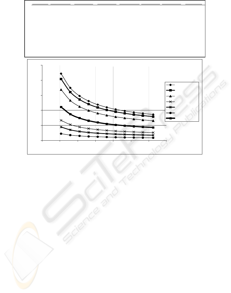
Intensity levels relative to the scene speed

100

150

200

250

10 20 30 40 50 60 70 80

Speed V [m/min]

Intensity levels

Object Min+

Object Max

Object Min-

Scene Min+

Scene Max

Scene Min-

Threshold

Figure 2: The influence on the intensity levels of the speed of the scene (acquisition frequency).

frames a priori acquired. The vision systems

dedicated to industrial applications can take the

advantage on the fact that the image environment

does not change a lot in time. In this way it can be

initially reserved a certain time for acquiring a large

enough number of image frames in order to be able

to identify the permanent characteristics of the

environment. All the intensity level distortions

present permanent characteristics. Using this method

is a necessity for the artificial vision systems

dedicated to applications where the errors on

binarization are not acceptable. In the applications

dedicated exclusively to shape recognition the errors

are accepted in a predefined range.

4 BINARIZATION THRESHOLD

VALUE AFFECTED BY THE

ACQUISITION FREQUENCY

ON THE

In moving scene applications, in order to maintain a

constant resolution of the vision system along the

direction of the scene movement, it is necessary the

ratio between the acquisition frequency (the image

lines rate – in the case of a line scan camera) and the

scene speed to be constant. The acquisition

frequency determines the exposure time of the CCD

sensor cells. It can be notice an important influence

of the speed (of the conveyor) on the intensity level

of the same image element in the same lighting

environment. In Figure 2 are presented the

experimental results obtained analysing the

influence on the intensity levels (for both: bright

object and dark background) of the speed of the

conveyor (acquisition frequency). The results were

obtained on a statistical population from an image

element on each measured speed. The second

column represents the measured speed of the scene

(conveyor) – V [m/min]. The 3

to 8

columns

represent image intensity levels estimated from the

analysed statistical population (temporal histogram).

The values from the Threshold column are the

binarization threshold values obtained from a global

optimum temporal thresholding method applied on

the histogram built for each analysed level of the

speed. In Figure 3 are presented graphical the

explanations on the meanings of the data involved in

the analysis of the influence of the speed

A NEW APPROACH OF GRAY IMAGES BINARIZATION FOR ARTIFICIAL VISION SYSTEMS WITH

THRESHOLD METHODS

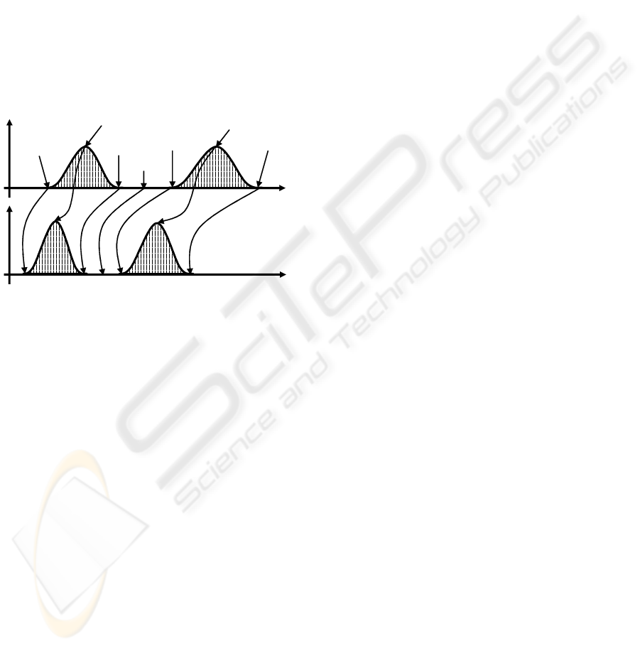
(acquisition frequency) on the intensity levels. The

artificial vision system benefits from these results

using a relation between the value of the binarization

threshold and the speed V of the scene

T = T (x, V) (18)

Because of the response time restrictions

imposed to the artificial vision system, instead of

using an explicit expression of the estimated

function T(x, V), a search method in an a priori filled

table (at set-up time) is more appropriate. The size

of the table is 256 (the number of the possible values

of the binarization thresholds), containing floating-

point values of the speed of the conveyor

(acquisition frequency) for which the value of the

binarization threshold has to be changed.

Object Min-

Object Min+

Scene Min-

Scene Min+

Scene Max

Object Max

Threshold

Increased speed

influence on

intensity levels

Intensity level

umber of

pixels

umber of pixels

Figure 3: The influence of the speed on the intensity

levels.

5 CONCLUSIONS

For the class of artificial vision systems dedicated

for inspection and measurement industrial

applications the error on binarization process is not

acceptable. In this, case classic methods like global,

local and dynamic threshold are not applicable. The

paper introduces a new approach of gray level image

binarization – temporal thresholding. For the class of

artificial vision systems dedicated for moving scene

the acquisition frequency is dependent on the speed

of the transmission support (usually a conveyor). To

solve this problem, the artificial vision system has to

estimate the influence of the acquisition frequency

on the histogram and on the binarization threshold

values. The paper proposes a processing time

efficient method to estimate the binarization

threshold for the case of an error free vision system

in the case of variation of the acquisition frequency.

REFERENCES

Haralick, R., Shapiro, L. (1992) Computer and Robot

Vision, Addison-Wesley Publishing Company.

Borangiu, Th, Hossu A., Croicu, A. (1994) -

ROBOTVISIONPro, Users Manual, ESHED

ROBOTEC, Tel – Aviv.

Croicu, A., Hossu, A., Dothan, E., Ellenbogen, D., Livne,

Y. (1998)- ISCAN-Virtual Class based Architecture

for Float Glass Lines, IsoCE’98, Sinaia.

Hossu, A., Croicu, A., Dothan, E., Ellenbogen, D., Livne,

Y.(1998) - ISCAN Cold-Side Glass Inspection System

for Continuous Float Lines, User Manual, Rosh-

Haayn.

ICINCO 2008 - International Conference on Informatics in Control, Automation and Robotics