
ON THE SAMPLING PERIOD IN STANDARD AND FUZZY
CONTROL ALGORITHMS FOR SERVODRIVES
A Multicriterial Design and a Timing Strategy for Constant Sampling
Dan Mihai
University of Craiova, Decebal Blvd, 107, Craiova, Romania
Keywords: Sampling period, PI algorithm, Fuzzy control, On-line timing, Servodrives.
Abstract: The paper deals with the best choice for the control sampling period in term of a multicriterial conditioning,
with the on-line timing and with a comparison between the conventional (like PI) control algorithms and the
fuzzy control. Several useful relations are followed by diagrams obtained in simulation and by different
real-time recordings both for the timing and for characteristic variables of the system. Implementations with
microcontroller and DSP are used for analyzing the design criterion and the timing strategy. The application
field concerns a servodrive, so the real-time constraints are quite strong. The author conceived a general
control strategy for the on-line timing based on imbricate interrupts, each pulse encoder acting on the
hardware input interrupt of the control processor.
1 INTRODUCTION
The sampling frequency plays an essential role in
implementing a digital control algorithm in real-
time, especially for the fast systems. Most of the
reference books give evaluations only for the upper
limit of the sampling period (T), as if the ideal value
would be as little as possible – only the capacity of
the control processor being the constraint. The
efficient choice of the sampling rate in closed-loop
system is based on its influence on the performance
of the control system. The absolute lower bound to
the sample rate is set by the system bandwidth. The
classical controllers (and their loops) are not robust
and their tuning (including the additional T
parameter) - although stated as well settled (Astrom,
1997), seems to be very difficult in complex
conditions. Not a few applications and studies
concern the sampling period design for different
kind of fuzzy control. An earlier idea (Coleman,
1994) about the robustness comparison between
fuzzy logic, PID control and sliding mode control,
will be extended now in the area of the control
sampling period.
During the last decades, the electrical drives
field has integrated more and more design
techniques, fast control processors and acquisition
modules for high performance platforms. A hybrid
approach is to have an inner current loop monitored
by a fuzzy controller (Mrozek, 2000) while the main
speed loop is monitored by a classical PI controller.
Another approach is to design a self tuning fuzzy
logic controller, based on some desired output
behaviour and hence, does not requiring a precise
model of the machine (Ibbini, 2002). Sometimes, the
results are quite close in term of performance (in
steady state or dynamic regime) but the
implementation effort is much lower for the fuzzy
solution (Silveira, 2002). Industrial equipment support
from few kHz to 20 kHz sample rate for the velocity
loop. This high rate of sampling combined with the
velocity observer, allows equipment to provide a very
fast control for industrial servo drives. Despite the
availability of several high performance DSP
controllers, many researchers are interested in
designing optimal control algorithms based on low-
cost solutions; such approach is typical for linear and
sliding-mode controllers designed for a DC servo
drive with a microcontroller and low sampling rate,
typical for embedded systems (Kosek, 2007).
The author developed a general on-line timing
for all digital control algorithms for the servodrives
with a hardware position loop and a software one for
the speed, proposing several relations for the
multicriterial correlation of the involved parameters,
T included. Several such relations require the T
value to be superior to some threshold limits.
72
Mihai D. (2008).
ON THE SAMPLING PERIOD IN STANDARD AND FUZZY CONTROL ALGORITHMS FOR SERVODRIVES - A Multicriterial Design and a Timing
Strategy for Constant Sampling.
In Proceedings of the Fifth International Conference on Informatics in Control, Automation and Robotics - SPSMC, pages 72-77
DOI: 10.5220/0001477600720077
Copyright
c
SciTePress
2 THE SERVODRIVE AND THE
ON-LINE CONTROL TIMING
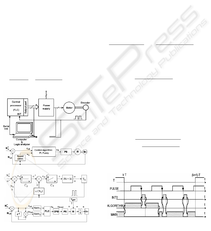
Figure 1a presents the main parts of the system.
Each encoder pulse acts on the interrupt entry of the
processor. The next control strategy and the timing
remain the same for any motor (and its associated
power supply), for different kind of control
algorithms (standard, fuzzy). The general systemic
structure is given by figure 1b; figure 1c is for a
conventional control and the next one (1d) presents
the fuzzy control. The main notations: N
α
*,N
αk
-
position set-point and the real position, in encoder
pulses; ε
αk
, Δε
αk
: position error, its variation referred
to a sampling period; ΔN
αk
- pulses encoder during
T; c
k
, c
kout
- the computed control and its outputted
value; Norm
i
: normalization blocks for each Fuzzy
Logic Controller (FLC); CPB: Control Processing
Block; PS - Power supply with digital control input;
T
gen
- torque generator; M - motor; En - encoder.
The encode has N
p/r
pulses per revolution and the
speed is monitored through a software image:
ksp
r/p
kdiv1kk
ks
Nc
TN
Nk2
T
Δ⋅=
⋅
Δ⋅⋅π
=
α−α
≈ω
−
(1)
Figure 1: The drive with different controllers.
k
div
is a division / multiplication factor for encoder
pulses. The real-time control strategy is based on 2
imbricate interrupts – figure 2. INT0 is a high level
priority interrupt generated by encoder pulses (the
falling edge). The low level priority interrupt is
software generated, marking the sampling period -
T. PULSE means the encoder signals. For standard
or non-conventional control algorithms, T must be
correlated with: a. the specific system dynamic; b.
n
min
- the minimum accepted value of the real speed
for which ω
k soft
is detectable; c. n
lw
- the size of the
data word (register) for ω
ks
; d. the accepted
resolution for the speed; e. the program length of the
on-line processing; f. The amount of memory
available for on-line recordings. b., c and d. give the
next restrictions for T:
[RPM]n
p/r
N
div
k)
lw
n
(
T
[RPM]n
p/r
N
div
k
max
6012
min
60
⋅
⋅⋅−
≤≤
⋅
⋅
(2)
When the range speed covers a full data register, for
having 1 LSB at minimum speed, T must be:
(2 -1) 60
[]
max
/
n
reg
k
div
T
N
nRPM
pr
××
≥
×
(3)
The e. condition generates another constraint for T
(Mihai, 1999). INT0 requested by the falling edge
encoder pulses computes ε
αk
, ΔN
k
and needs the
time-Δt
INT0
. Δt
av.instr.
is the average time for a
processor instruction. Having the code program
length for the software interrupt routine-N
max.ALG. instr.
imposed by the algorithm, T must be:
div
INTrp
instravinstrALG
k
tNn
tN
T
⋅
Δ⋅⋅
−
Δ⋅
≥
60
1
0/max
...max
(4)
As for f. condition, the data memory space for all
on-line records is given by the number of data bytes
Figure 2: The proposed timing for on-line control based on
interupts.
a.
b
.
c.
d.
ON THE SAMPLING PERIOD IN STANDARD AND FUZZY CONTROL ALGORITHMS FOR SERVODRIVES - A
Multicriterial Design and a Timing Strategy for Constant Sampling
73
n
Bytes
saved for each T and the regime duration Δt
pos
.
A too much little T can lead to an outrunning of the
available memory space V
data mem.
. Then:
.
max.
memdata
Bytespos
V
nt
T
⋅Δ
≥
(5)
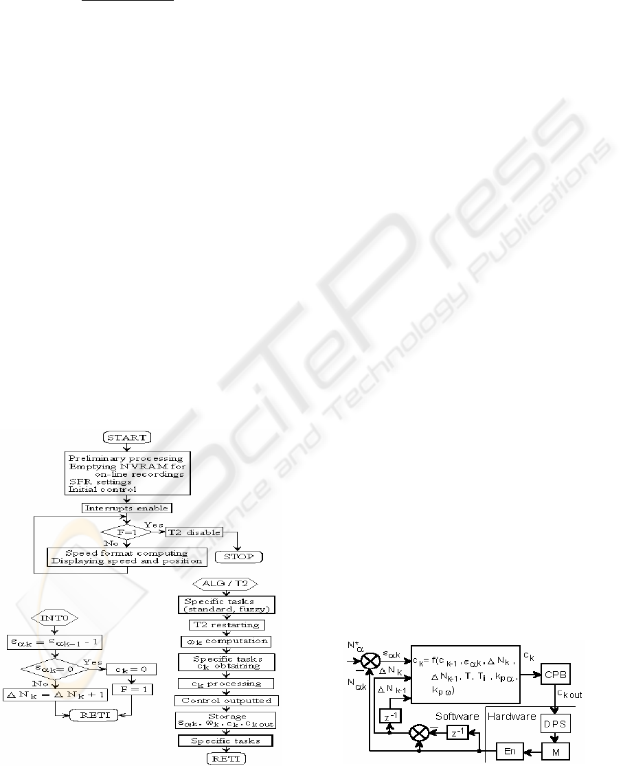
The basic software structure for the on-line control
is presented in figure 3. The main program performs
an initial preparation of the interrupt system and T2
timer. Then, the interruptible loop makes some
auxiliary processing concerning data displaying and
a test for the flag F which signals a null position
error. Main tasks are those monitored by the
hardware interrupt INT0 and the software interrupt
ALG / T2. The first is a very fast one and is
absolutely the same for all type algorithms, which
control the position and speed. A more complex
interrupt routine is ALG / T2. The specific tasks
concern some additional computing procedures for
the control c
k
and a characteristic up-to-date for
addresses content allocated to regressive variables of
standard algorithms. The processing of the obtained
control means the extraction of one effective control
c
k out
in 8 bit format which acts on a power supply.
2.1 Standard Digital (Micro)
Controller
The author combined the computations for both
loops into a single relation for the control:
Figure 3: Flow chart of the on-line control program.
c
k
= c
k-1
+ k
p
ω
·(
ε
ω
k
− ε
ω
k-1
)+ k
p
ω
·T·
ε
ω
k
/ T
i
(6)
k
pα
, k
pω
and T
i
are the tuning parameters of position
and speed loops. Figure 4 has a more detailed
systemic structure of the figure 2a. The next form
was obtained as an on-line optimal one:
c
k
= c
k-1
+ A·
Δ
N
k-1
+ B·
Δ
Nk + C·
ε
α
k
(7)
A = k
p
ω
· c
sp
; B = - k
p
ω
· c
sp
·( k
p
α
+
T / T
i
)
(8)
C = - k
p
ω
· k
p
α
· T / T
i
A, B and C are the new tuning parameters and all
other variables are delivered by INT0. The real-time
implementation was prepared by various simulations
on a model having the structure and the
characteristics very close to the real operation and
capabilities of the system and of the microcontroller.
The algorithm was applied for simulation and on-
line control for a drive system with: a 12 V DC
brushed low-inertia motor; an 8 bits microcontroller;
an encoder with 2500 lines / rev. A multicriterial
optimal conditioning (Mihai, 1999, 2004) of the
involved data meant T = 2.456 ms and c
sp
= 1.02 ≅1
(an ideal value). The figure 5 presents the simulation
results by the main macroscopic variables. The on-
line results are those from figure 6, the behaviour
being like the expected one by simulation. Some
differences are in connection with a particular
strategy for the pre-final time segment (Mihai,
2004). Figure 7 is a witness of what is happening in
real-time, the analyser recordings giving details for
the timing (including the T value, interrupt events)
and for precise evaluations for each activated task.
Notations: SPER-sampling period; PULSE- encoder
pulses; INT0-external interrupt service routine;
PROC-all speed loop tasks; ARITH- arithmetic
routines; SCON-control tasks. Figure 7a reveals the
timing for a low speed and the total processing time
for having a control: 452 μs. The next diagram is for
the rated speed and the real T - 2.47 ms. 7c makes a
precise evaluation of the final position error: 2.5
pulses, that meaning 1 / 1000 rev. during 11.37 ms.
Figure 4: For the standard control algorithm.
ICINCO 2008 - International Conference on Informatics in Control, Automation and Robotics
74
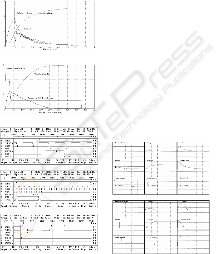
Fig. 8 is for T= 2.456 ms (the ideal value) and T =
1ms. It can be seen the worsening of the
performance; the control is saturated and a big
position overshoot is present. So, a lower T value
does not bring a higher performance.
Figure 5: Simulation results / standard algorithm.
Figure 6: Real-time results / standard algorithm.
a
b
c
Figure 7: The on-line tasks / standard algorithm.
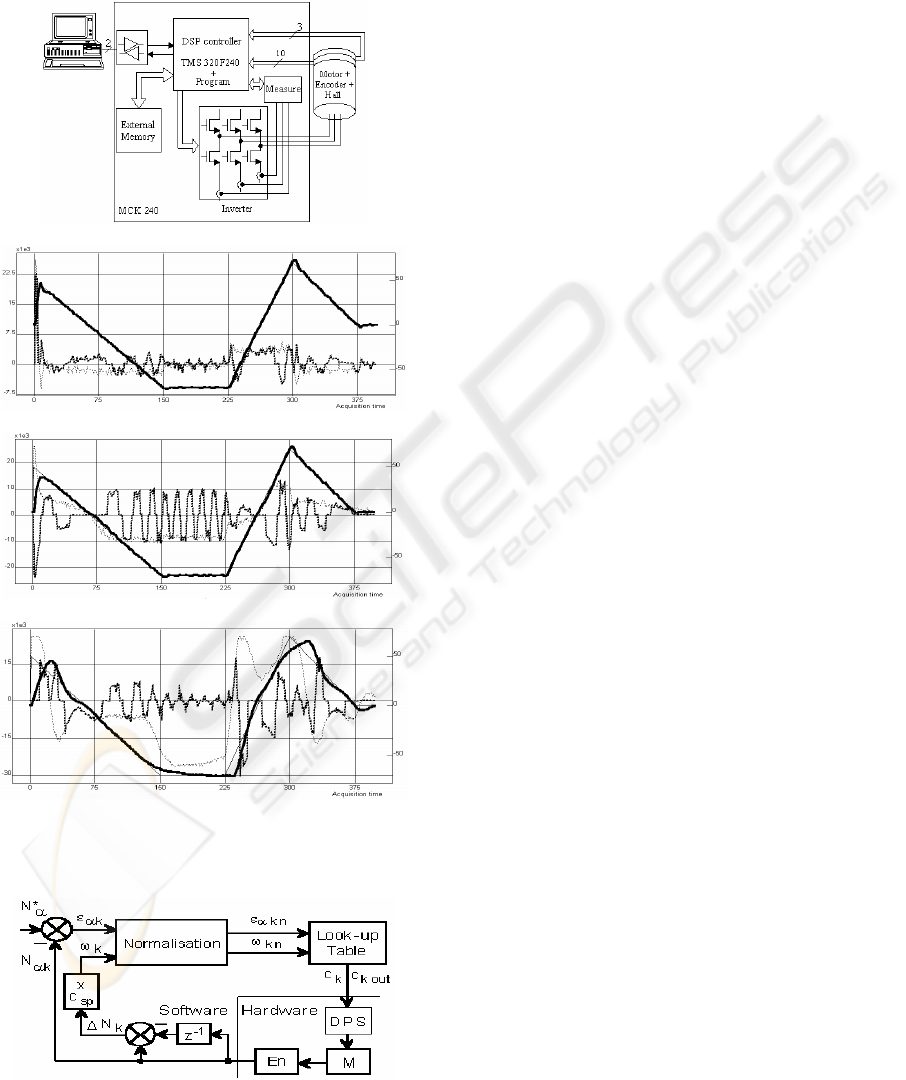
2.2 Standard Algorithm by DSP
Controller
The first idea for improving the bad results from fig.
8b is to use a much more performing hardware. The
next experiment was made with a brushless DC
motor and a DSP controller (Technosoft, 1997). The
figure 9a presents the system. The results (in real-
time) from figure 9b are for no-load conditions. The
figure 9c proves a good general tuning when the
motor has a load. This first two result sets were for
T=1 ms (speed loop) and T=0.1 ms (current loop).
With a faster control sampling (twice), the results
are loosing the quality-fig. 9d. A good choice for T
is better than an expensive hardware solution.
2.3 A Fuzzy Digital Controller
The input variables for the FLC are:
ε
α
nk
= (N
α
*- N
αk
) ·
ε
α
nk max
/ N
α
* ≥ 0 (9)
Δ
ε
α
nk
=
ε
α
n k
-
ε
α
nk-1
=
Δ
Nk·Δ
ε
α
nk max
·c
sp
/
Ω
max
≤ 0 (10)
The most reduced on-line computational effort is
obtained using a look-up table (LUT) filled off-line.
Fig. 10 gives the image of the equivalent systemic
structure of FLC. The control values are stored by
the columns concatenation of a matrix with the final
control values, so the additional software block CPB
is no more necessary. The fuzzy LUT strategy was
a
b
Figure 8: T = 2.456 ms (a) and T = 1 ms (b).
ON THE SAMPLING PERIOD IN STANDARD AND FUZZY CONTROL ALGORITHMS FOR SERVODRIVES - A
Multicriterial Design and a Timing Strategy for Constant Sampling
75
applied for the same servodrive as for 2.1. The main
characteristic elements are presented by fig. 11. The
notations: az-almost zero; vs-very small; s-small; rs-
relative small; m-medium; b-big; vb-very big. The
off-line tuning for the fuzzy rule base was made by
a.
b.
c.
d.
Figure 9: The real-time results for a standard algoritm and
a DSP controller.
Figure 10: A LUT based FLC.
simulation on model, with the results from the figure
12. The on-line results are depicted in figure 13 and
the on-line timing is given by the figure 14. It can be
notice a good concordance between the simulated
and the real-time results. The meaning of the
additional notations used by the figure 14: NORM-
normalization task; LUT-searching in look-up table.
The apparent discrepancy between the position
smooth evolution and the speed diagram is explained
by the fact that the software image ΔN
k
is a
truncated value for speed, while the real speed and
the position support a filtering effect of mechanical
inertia. The ringing of the control is, basically, a
result of fuzzy rules commutation. The control
variable evolution (motor voltage) reveals a very
sensitive behaviour of the controller, better than for
the standard controller–the figures 5 and 6. The
quality of the whole evolution is also presented in
the (ε
α
, ω) state-space coordinates, with a good
(smooth) behaviour and an entry with very low
speed in the proximity of the final point. The same
sampling control period as for the standard control
algorithm was used: T = 2.456 ms, according to the
same multicriterial optimum. It is confirmed the
right operation of the 2 interrupts and the existence
of quite large time reserve during each T for
additional tasks. The diagram from the figure 14a
concerns a quasi steady state regime, revealing the
typical task distribution. Several values for the tasks
time are precisely measured. Δt SPER = 2.456 ms
<< T
m
= 50 ms (the electromechanical time constant
of the motor); Δt PULSE = 125.5 μs - for a speed of
192 RPM. The last diagram caught the final
algorithm time segment. The final detectable speed
is 3.39 RPM. After the T2 timer (that marks the
sampling rate and the cyclic processing for the
control determination) is disabled, it can be seen a
single pulse coming from the encoder. It is the ideal
position error and the real too. Other durations are:
Δt INT0 = 10 μs; Δt PROC = 558 μs < 25 % x T; Δt
NORM = 310.5 μs; Δt LUT = 20.5 μs; Δt SAVES =
26 μs (globally). The most of time is necessary for
the normalization arithmetic operations.
3 CONCLUSIONS
The sampling control period is more than additional
tuning parameters for the digital control. The author
conceived a multicriterial conditioning relation set
with the limitation both for the upper and the lower
values for the sampling period. The general timing
proposed for the servodrive control is based on
imbricate interrupts. A strong real-time constraint is
accomplished by a hardware interrupt that makes an
acquisition rate different than the control rate. The
ICINCO 2008 - International Conference on Informatics in Control, Automation and Robotics
76
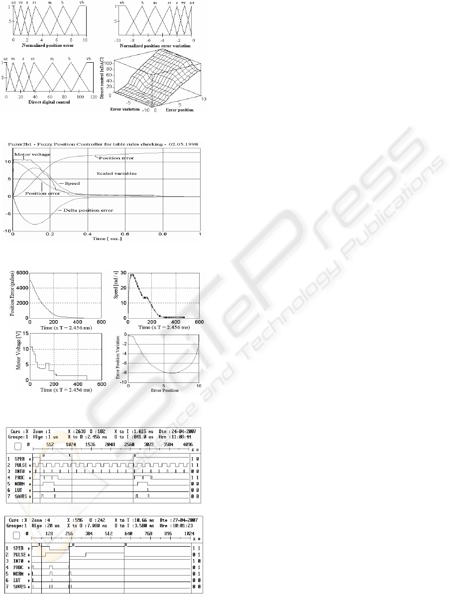
Figure 11: The basic elements for a LUT - FLC.
Figure 12: Results for a FLC in simulation.
Figure 13: On-line results for a LUT based FLC.
a
b
Figure 14: The on-line recordings for a LUT FLC.
on-line results, both for the standard algorithm and
the fuzzy control, are very good in terms of the
macroscopic variables and for the timing revealed by
on-line recordings with a logic analyzer. Some
experiments proved that a good choice for the
sampling control period is not necessarily related
with a high end control processor but is the result for
all correlations previously mentioned.
REFERENCES
Astrom, K.J., Wittenmark, B., 1997. Computer-controlled
systems: theory and design, Prentice Hall, USA.
Coleman C. P., Godbole D., 1994. A Comparison of
Robustness: Fuzzy Logic, PID and Sliding Mode
Control, Proc. of the American Control Conference,
pp. 1654-1659.
Do Wan, K., Jin Bae, P., Young Hoon, J., 2007. Effective
digital implementation of fuzzy control systems based
on approximate discrete-time models, Automatica
(IFAC Jour.), Volume 43 , Issue 10, pp. 1671-1683.
Ibbini, M.S., Jafar, A.S., 2002. Self-Tuning Fuzzy Logic
Controller for a Series DC Motor, Proc. (369) Power
and Energy Systems, Acta Press.
Kozek, M., Lorenz, A., Kampas, Ph., 2007. Modeling and
control of an electric servo drive with strong
restrictions in the control variable, Int. Journal of
Applied Electromagnetics and Mechanics, Vol. 25,
Number 1-4, pp. 521 – 527.
Mihai, D., Constantinescu C., 1999. Fuzzy Versus
Standard Digital Control for a Precise Positioning
System with Low-Cost Microcontroller, PCIM99,
Nurnberg, Proceedings, pp. 249-255.
Mihai, D., 2004. Systèmes d’entraînements électriques I.
Problèmes fondamentaux. Systèmes avec moteurs à
courant continu, Ed. Universitaria, Craiova.
Mihai, D., 2006a. Additional Mathematical Pre-processing
for the Fuzzy Control of a Servodrive, WSEAS Trans.
on Circuits and Systems, Is. 11, Vol. 5, pp. 1575-1580.
Mihai, D., 2006b. An Optimized Fuzzy Control Algorithm
for Servodrives. Some Real-Time Experiments.
Proceedings, IS ’06, London, paper 1-4244-0195-
X/06-CD ROM, pp. 192-197.
Mrozek, B, Mrozek, Z., 2000. Modelling and Fuzzy
Control of DC Drive, ESM 2000, Ghent, pp186-190.
Silveira, P. E., Souza, J.R., Biazotto R. de, V. M., 2002.
Speed Control of an Autonomous Mobile Robot:
Comparison between a PID Control and a Control
Using Fuzzy Logic, J. Braz. Soc. Mech. Sci., vol.24,
no.2, pp.127-129.
Vas, P., 1999. Artificial-Intelligence-Based Electrical
Machines and Drives, Oxford University Press.
*** Technosoft S. A., 1997, MCK 240 DSP Motion
Control Kit. User Manual, Switzerland.
ON THE SAMPLING PERIOD IN STANDARD AND FUZZY CONTROL ALGORITHMS FOR SERVODRIVES - A
Multicriterial Design and a Timing Strategy for Constant Sampling
77
