
A NEW APPROACH FOR MODELING ENVIRONMENTAL
CONDITIONS USING SENSOR NETWORKS
Mehrdad Babazadeh and Walter Lang
Institute for Microsensors, -actuators and -systems (IMSAS), University of Bremen, Otto-Hahn-Allee, Bremen, Germany
Keywords: Temperature, relative humidity, air flow, estimation, grey-box, model.
Abstract: An approach to estimate environmental conditions (ECs), temperature, relative humidity and air flow in a
few desired sensor nodes in a wireless sensor network, slept for reducing battery-consumption or inactive
due to either empty batteries or out-of-range is presented. A nonlinear, multivariable model containing the
interconnections is extracted and using data of surrounding active sensor nodes is broken to the linear
models. Unknown parameters of the model are verified by a multivariable identification method. The
proposed approach is independent of the type of ventilation system. It can be used in different applications
such as designing model base ECs controllers as well as an estimator in fault diagnosis methods.
1 INTRODUCTION
Identification, modeling and control of Temperature
(T), relative Humidity (H) and air Flow (F) as the
environmental conditions (ECs) in the air
conditioned closed spaces have gained a lot of
attractions during the last few years. Therefore,
simple and precise mathematical models can play a
key role in these areas. Improving such linear
models or proposing new nonlinear models is very
vital on this issue. As the first step, we try to achieve
a simple mathematical model for the ECs using a
wireless sensor network established inside the
container loaded with freights. We utilize this model
to introduce a new technique to estimate the EC in
the place of some desired sensor nodes (DSNs).
They may be either in sleep mode or out of service.
As stated by the articles, there are three types of
models: based on (Sohlberg, 2003), White-box
models are made of theoretical considerations where
the grey-box models are extracted from the first
principles and parameters of the models are obtained
by measurement and black-box models are identified
only using measurement of the system input and
output. The methods achieved to the white, grey and
black-box models of T for air-handling units have
been addressed in
(Ghiaus, 2007) , (Shaikh, 2007),
(Brecht, 2005), (Desta, 2004), (Frausto 2004)
. Some
other works consider the effects of air flow pattern
on the T in special cases
(Moureh, 2004), (Rouaud,
2002)
and (Smale, 2006) is a brief review of numerical
models of airflow in refrigerated food applications.
(Desta, 2004) outlines a method to achieve an
accurate model of T in a closed space using both k-ε
model and a data-base mechanistic (DBM) modeling
technique. It doesn’t consider the effect of the heat
transfer from the neighboring zones.
All previous models are obtained between input
(inlet) and a point of corresponding space. As
attested by these methods, the ECs inside the
container will change only due to variation in inlet.
Some of the models obtained in the existing papers
either linear or nonlinear don’t consider all of
important parameters of the ECs. Furthermore,
particular conditions and the limit range of the
parameter variations are necessary and despite the
high precision, complexity makes them impractical
in some applications.
If return to model making in the mentioned
space, nonlinear multivariable nature and
interconnections between the variables of the ECs in
addition to the presence of the freight as an
unpredictable, immeasurable disturbance, effects of
dynamic of flow, surfaces and walls inside the
container increase complexity of the model which
we are looking for. Another important factor is
disturbance which can be appeared in the different
ways and may be cause a big estimation error: (i)
Opening the door of the container; (ii) changing
either direction or rate of the air flow by some
obstacles; (iii) thermal or moisturize influences of
78
Babazadeh M. and Lang W. (2008).
A NEW APPROACH FOR MODELING ENVIRONMENTAL CONDITIONS USING SENSOR NETWORKS.
In Proceedings of the Fifth International Conference on Informatics in Control, Automation and Robotics - SPSMC, pages 78-83
DOI: 10.5220/0001477800780083
Copyright
c
SciTePress
some freight. All attempts in the first step of the
present research are towards introducing a grey-box
nonlinear model between inlet and one DSN. We
will use previous data of a deactivated sensor in
addition to the present and previous data of some
surrounding sensor nodes to estimate unknown
parameters of the related simplified models.
According to fig. 1 and also our main proposal in the
energy management of the wireless sensor network,
there will be a few special key sensor nodes (KSNs)
those will send some specific information to main
processor and or to the other sensor nodes. The
KSNs should be in active mode during the normal
operating mode. The KSNs have three major
functions: (i) they measure environmental conditions
alternatively; (ii) they evaluate measured values and
do some estimation of the ECs in the DSNs and
update previous models after measuring and
receiving some new data; (iii) they will deactivate
DSNs when the operational conditions are normal
and there are no big changes in the ECs. Usually a
while after loading the container, the ECs inside the
container have less variations. This duration is the
best time to utilize the method to take more DSNs to
sleep mode and to estimate the ECS instead of the
direct measurement. The KSNs can be located
everywhere inside the container, even near the door
or near to the inlet. If they are located in some key
points, mismatch error due to no considering
unpredictable phenomenon will be avoidable
because depending on the floating input approach,
uncertainties and disturbances are considered
indirectly as the input change. It is also independent
of the type of the ventilation system. Useful
reference for sensor networks is (
J. Elson, 2004).
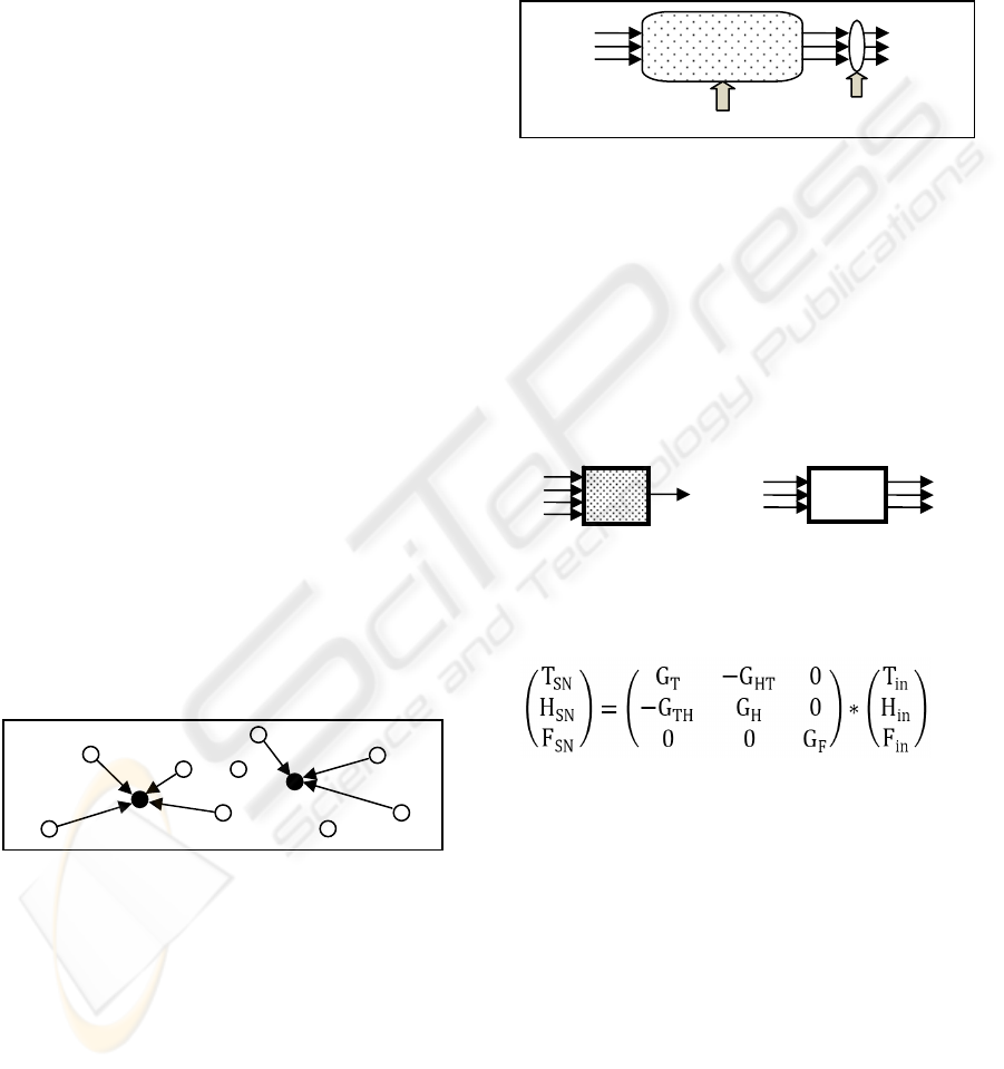
Figure 1: Proposed sensor network.
2 PROBLEM FORMULATION
Fig. 2 shows a general scheme of the system, inside
the container between the inlet and a spatial position.
It is a complicate, time and place dependent, multi-
variable system. It consists of three inputs, three
outputs, disturbance and noise. Due to the coupling
in the ECs, doing independent experiments in the
actual container is difficult. It completely depends
on the initial conditions so that a change in the T or
relative humidity of the inlet may change both T and
H in all positions of the space. Variation in the rate
of input air flow changes the measurement results
and disturbance may change all the results so that
based on the existing conditions, measured values
might be different even in the same place.
Figure 2: Schematic of Container as a MIMO model.
Floating input approach identifies multivariable
models between the KSNs and the DSNs, not
between the inlet and a DSN. Every non modeled
disturbances which excite some KSNs, is modeled
as an implicit input change, not a pure disturbance.
Now, the new input nodes (KSNs) in the defined
multi-input and single-output (MISO) system change
output nodes (DSNs). Fig. 3 shows K1, K2, K3 and
K4 as the KSNs and S1 as the DSN.
Figure 3: Models between the KSNs and a DSN.
The first step for modeling is using linear transfer
function matrix. Without considering noise we have:
(1)
(T
SN
, H
SN
and F
SN
) and (T
in
, H
in
and F
in
) are
respectively measured value of (T, H and F) in SN
and inlet. Whereas T and H have opposite effects on
each other, we assign negative sign for the
interconnection. It is assumed that F has no direct
effect on the steady state values of T and H, but it
influences on the speed of their variations. However,
the effect of F are included in all G
T
, G
H
, G
HT
and
G
TH
(which are transfer functions between different
parameters of the ECs) with some exponential
functions that we will mention later. To investigate
validity of the model we employ a reverse lemma
and some assumptions in different border conditions.
Assumption 1, steady state values of T and H:
S1
MISO
K1
K2
K3
K4
{
T
H
F
T
H
F
MIMO
K
1
S
1
}
Input (inlet):
Temperature
Humidity
Flow
Output (SN):
Temperature
Humidity
Flow
Noise
Disturbance
Multivariable
Syste
m
K1
K5
K3
S2
K6
K7
K2
K4
S1
A NEW APPROACH FOR MODELING ENVIRONMENTAL CONDITIONS USING SENSOR NETWORKS
79
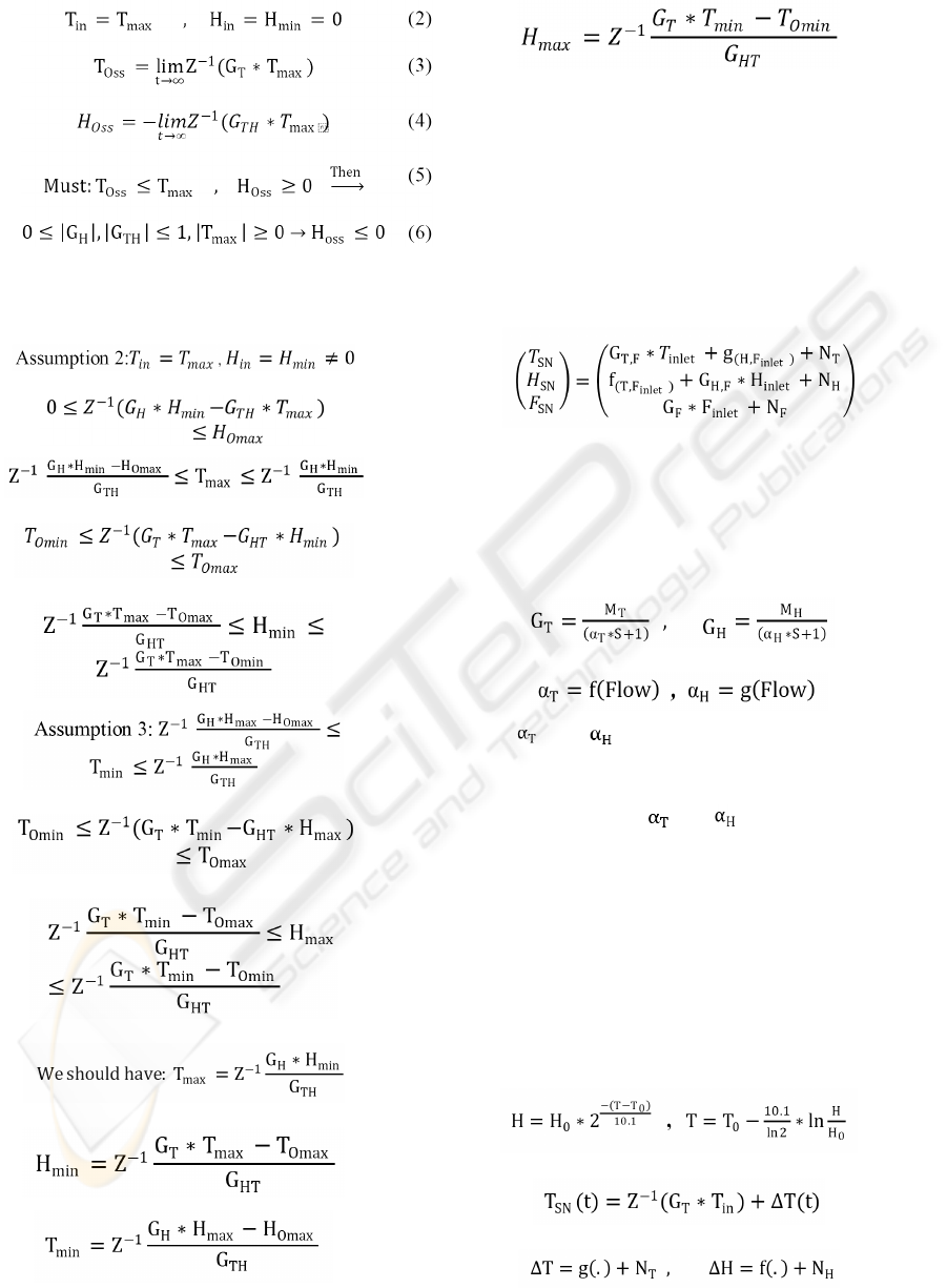
It can’t be correct because, negative H can’t be
occurred. We consider some permissible margins so
that T and H locate in the mentioned margin:
(7)
(8)
(9)
(10)
(11)
(12)
(13)
(14)
(15)
(16)
(17)
(18)
Having H
min
and H
max
, other input limitations
will be verified. Then there are the specific bands for
inputs so that outputs of linear model will be located
in the admissible areas. Accordant with the lemma,
linear model (1) can’t be a proper model. The
nonlinear model will be made based on the basic
knowledge of the nonlinear nature of the
interconnections. Considering some linear transfer
functions for direct effects and obtained nonlinear
functions for the interactions, we have:
(19)
g(.) and f(.) are nonlinear interconnections
between T and H which are influenced by F. As
stated by
(Ghiaus, 2007) and (Zerihun Desta, 2004),
model of T can be a first-order transfer function. We
also use the effect of the parameters with the same
dimensions in the following:
(20)
(21)
and illustrate speed of the responses and
M
T
and M
H
steady state values of T and H. They
74have reverse relation with F. Then, the further
flow rate, the less
and . The SNs can detecte
variations in the ECs showed by ∆T, ∆H and ∆F.
If the position of the SNs is close, we can assume
that all models in mentioned MISO system, showed
in fig. 3 are independent. It can be considered as
several single-input and single-output (SISO)
systems. Now, they should be combined using a
multivariable identification method. Accordant with
the thermodynamic relations, with 10.1 ºC
increasing T, H will be reduced to the half and we
have:
(22)
(23)
(24)
ICINCO 2008 - International Conference on Informatics in Control, Automation and Robotics
80
(25)
(26)
(27)
Z
-1
is unit delay in field of Z transform. It is
probable that the amounts of T
oss
and H
oss
are
changed because of the variation in air flow pattern.
However, we consider it on the transfer functions G
T
and G
H
when running the on-line estimation. From
previous results, we will derive a time dependent,
nonlinear, multivariable matrix equation and a
function of the several KSNs. Uk is a function to
obtain the effects of the KSNs on a DSN.
(28)
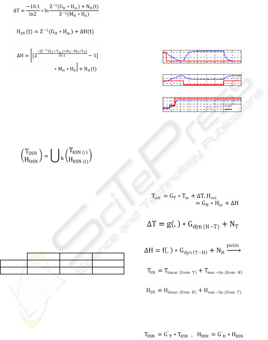
3 SIMULATIONS
Results of the SISO system with initial conditions in
the table 1 has been shown in fig.4. It is noted that a
part of the parameters such as time constant of T in
simulations have been inspired of actual behavior of
a real experiment and the rest are based on primary
assumptions of the authors.
Table 1: Initial conditions for inlet and S1.
T
0
H
0
F
0
inlet 10 30 15
DSN(S1) 9 28.5 13.5
According to fig. 4 Set points of T at 2000, H at
(12000 and 35000) and F at (4000 and 7000)
seconds change. An obstacle as a disturbance
changes the rate of the air flow and influences on the
speed of the responses. However, it will not change
the steady state value of the ECs. The initial
conditions of T and H in output are different with
those in input (inlet) and after changing T in input,
output changes slowly to a new equilibrium point
because the amount of flow is low in the beginning.
At 4000 and 7000 seconds air flow increases
respectively to F
max
/2 and F
max
and immediately the
responses of T and H become faster. When H in inlet
does not change, H in output changes only due to
changing T in output. There is a similar story for T
in output independent of T in input which varies
with the variation of H in output. Dashed curves
show the ECs in a desired place inside the container.
0 0.5 1 1.5 2 2.5 3 3.5 4 4.5
x 10
4
0
5
10
Temperatures using nonlinear model
Temperature (C)
time (sec)
0 0.5 1 1.5 2 2.5 3 3.5 4 4.5
x 10
4
20
40
Relative Humidities using nonlinear model
R. Humidity (%)
time (sec)
0 0.5 1 1.5 2 2.5 3 3.5 4 4.5
x 10
4
10
20
30
40
50
Air flow using nonlinear model
Flow(m/s)
time (sec)
Sensor
Inlet
Figure 4: ECs in SN when the ECs in input change.
4 AN INDIRECT SOLUTION
We employ the advantages of the sensor network
and introduce floating input approach. We assum
that m numbers of the KSNs are measuring the
conditions when input is inlet and we have:
(29)
(30)
(31)
(32)
(33)
We can suppose that the nonlinear
interconnections from the inlet are both in the KSNs
and the DSNs. Then, we can remove these parts
when we consider the KSNs as the input:
(34)
G´
T
, G´
H
are the linear transfer functions
between a KSN and a DSN and its unknown
parameters should be verified using a system
A NEW APPROACH FOR MODELING ENVIRONMENTAL CONDITIONS USING SENSOR NETWORKS
81
identification technique. Now, we will have some
SISO matrix equations which should to be solved. M
and P are functions for combining linear effects. We
use them in the identification method, indirectly. U
Ti
and U
Hi
are new inputs, in the m numbers of the
KSNs. G´
Ti
and G´
Hi
are linear transfer functions of
T and H, written between the KSNs and the DSN.
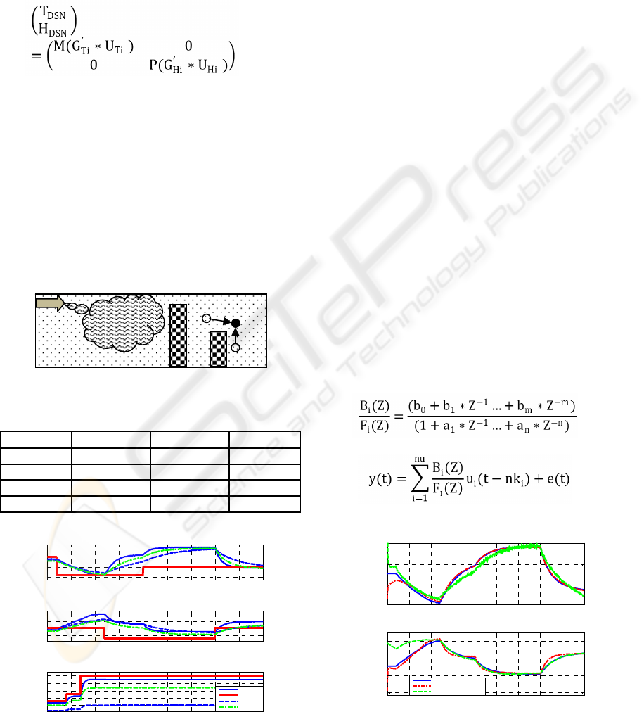
(35)
5 RESULTS
As an example, showed in fig. 5, there are two KSNs
and one DSN attached to the walls, there are some
obstacles so that the change-rate of the ECs near to
the SNs is different with those in inlet. There are
also different amounts of initial conditions for
different SNs because of their positions or
corresponding measurement errors (table 2). The
simulation results has been shown in fig. 6.
Figure 5: A container with inlet, KSNs and DSN.
Table 2: Initial conditions.
T
0
H
0
F
0
inlet 10 30 15
K1 9 28.5 13.5
K2 8.5 27 3
S1 8 25.5 10
0 0.5 1 1.5 2 2.5 3 3.5 4 4.5
x 10
4
0
5
10
15
a. Temperatures of K1, K2 and S1 using nonlinear model
Temperature (C)
time (sec)
0 0.5 1 1.5 2 2.5 3 3.5 4 4.5
x 10
4
20
40
b. Relative Humidities of K1, K2 and S1 using nonlinear model
R. Humidity (%)
time (sec)
0 0.5 1 1.5 2 2.5 3 3.5 4 4.5
x 10
4
10
20
30
40
50
c. Flows of K1, K2 and S1 using nonlinear model
Flow (m/s)
time (sec)
K1
Source
K2
S1
Figure 6: Outputs when T, H and F in input change.
As shown in fig. 6, curves of K1, K2 and S1 are
according with the data extracted from models
introduced in equations (23) and (26) and curves
related to the inlet are the set points. The relations of
T, H and interconnections are updated based on the
amount of F at the related instant of the simulation.
6 OFF-LINE IDENTIFICATION
Refer to equation (35), there are separate MISO
systems for T as well as H. All unknown parameters
should be determined using an off-line identification
technique. Then, we assume that KSNs are active
and there is a failure on the DSN or it is in sleep
mode and having new inputs we will have the new
estimations of the ECs in the DSNs using existing
transfer functions. The temperature estimation
results have been shown in fig. 7 and fig. 8 with the
SISO and MISO models, respectively. To show
capability of the method, the results have been
plotted together with the previous results of the EC
in S1 from introduced nonlinear model. the
measured T of K1 in the vicinity of S1, without any
variation in T of inlet and K2. We obtain its effects
on S1 when estimated by K1 and K2 compare with a
regular estimation method using model obtained
from inlet-DSN. The Solid wide curves illustrates
nonlinear model output and dashed curves represent
obtained results separately using linear models and
then with MISO estimation using output error (OE)
method in system identification toolbox of Matlab:
(36)
(37)
0 0.5 1 1.5 2 2. 5 3 3.5 4 4.5
x 10
4
5
10
15
a. High order SISO Estimation
Temperature (C)
time (sec)
0 0.5 1 1.5 2 2. 5 3 3.5 4 4.5
x 10
4
10
20
30
40
b. High order SISO Estimation
R. Humidit y (%)
time (sec)
S1:Actual
S1:Estimate by K1
S1:Estimate by K2
Figure 7: Actual and estimated T and H, model with the
order three using K1 and K2, separately.
K1
K2
S1
Inlet
ICINCO 2008 - International Conference on Informatics in Control, Automation and Robotics
82
To achieve a desired speed and regard to the
nonlinear nature of the responses that we have still
in the SNs, we utilize a linear transfer function with
the order more than two. Whereas the higher order
models will cause some difficulties in the
application, we don’t use the order more than three.
Separate estimations using SISO models have less
accuracy than those using MISO models.
0 0.5 1 1.5 2 2.5 3 3.5 4 4.5
x 10
4
5
10
15
c. Multivariable High order model es timation
Temperature (C)
time (sec)
0 0.5 1 1.5 2 2.5 3 3.5 4 4.5
x 10
4
20
25
30
35
40
d. Multivariable High order model estimation
R. Humidity (%)
time (sec)
S1:Actual
S1:High order, Using K1,K2
Figure 8: T and H, actual, estimation using high order
multivariable model from K1, K2.
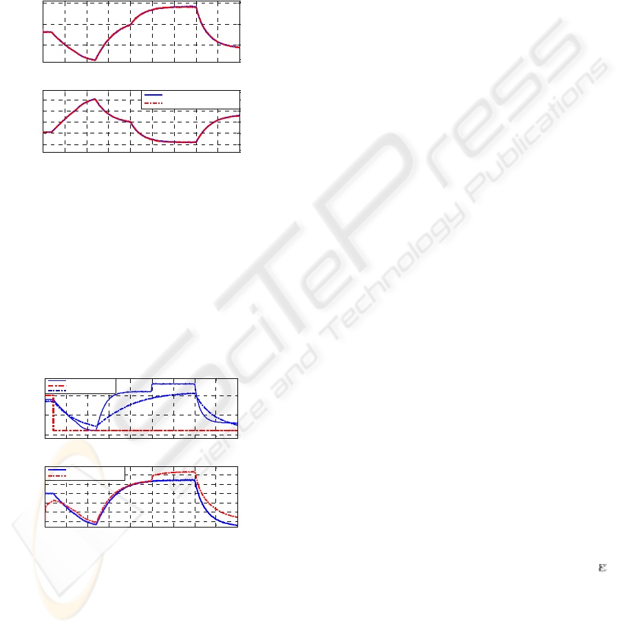
More important results are obtained when there
is a disturbance in vicinity of the SNs influences
some of the KSNs. fig. 9 shows the variation of T at
25000 seconds which affects both K1 and S1. Model
obtained from inlet-S1 can’t show this influence on
S1 because there are no influences on the inlet.
However, floating input method can estimate it
because at least one KSN senses it.
0 0.5 1 1.5 2 2. 5 3 3.5 4 4.5
x 10
4
0
5
10
a. Source and measurement results when there is a T disturbance on K1
Temperature (C)
time (sec)
K1: Measurement
T in inlet
K2: Measurement
0 0.5 1 1.5 2 2. 5 3 3.5 4 4.5
x 10
4
2
4
6
8
10
12
b. Disturbance effects with High order SISO model of K1-S1
Temperature (C)
time (sec)
S1:Estimated by inlet
S1:Estimated by K1
Figure 9: a. measured T in inlet, K1 and K2 and b.
estimation using inlet and K1with existing a disturbanc.
7 CONCLUDING REMARKS
This paper propuses a new hybrid model for
environmental conditions inside a container and
shows that it has much more accuracy for wide
range of parameter variations compared to other
conventional linear models between inlet and a
desired place. The new technique provides a
simplified multivariable model based on the
surrounding sensor nodes used for estimating the
ECs in the desired nodes. The simulation results and
mathematical proofs for different situations endorse
the capability of the proposed technique. At the end,
it should be noted that the comparison among
different multivariable estimation methods and their
implementations as well as finding the minimum
number and the best place of the KSNs are real
challenges main concerns on this issue.
REFERENCES
Ghiaus, C., Chicinas, A. and Inard, C., April 2007, ”Grey-
box identification of air-handling unit elements,
Control Engineering Practice”, Vol.15, Issue 4, pp.
421-433.
Shaikh, N. I and Prabhu, V., May 2007,”Mathematical
modeling and simulation of cryogenic tunnel
freezers”, Journal of Food Engineering, Vol. 80, Issue
2, pp 701-710.
Smale, N.J., Moureh, J. and Cortella, G., Sep. 2006, ”A
review of numerical models of airflow in refrigerated
food applications”, International Journal of
Refrigeration, Vol. 29, Issue 6, pp. 911-930.
Van Brecht, A., Quanten, S., Zerihundesta, T., Van
Buggenhout, S. and Berckmans, D., 20 Jan. 2005,
“Control of the 3-D spatio-temporal distribution of air
temperature”, International Journal of Control, 78:2,
pp. 88- 99.
Zerihun Desta, T., Van Brecht, A., Meyers, J., Baelmans,
M. and Berckmans, D., June 2004, ”Combining CFD
and data-based mechanistic (DBM) modeling
approaches, Energy and Buildings”, Vol. 36, Issue 6,
pp 535-542.
Frausto, H. U. and Jan G. Pieters, Jan.2004, ”Modeling
greenhouse temperature using system identification by
means of neural networks”, Neurocomputing, Vol. 56,
pp.423-428.
J. Moureh and Flick, D., Aug. 2004; ”Airflow pattern and
temperature distribution in a typical refrigerated truck
configuration loaded with pallets”, International
Journal of Refrigeration, V. 27, Issue 5, pp. 464-474.
Rouaud, O. and Havet, M., May 2002, ”Computation of
the airflow in a pilot scale clean room using K-
turbulence models”, International Journal of
Refrigeration, Vol. 25, Issue 3, pp. 351-361.
Sohlberg B., May 2002, Apr. 2003, ”Grey box modeling
for model predictive control of a heating process”,
Journal of Process Control, Vol. 13, Issue 3, pp. 225-
238.
J. Elson and D. Estrin. Sensor Networks: A Bridge to the
Physical World, chapter 1. Wireless Sensor Networks.
Kluwer Academic Publishers, 2004.
A NEW APPROACH FOR MODELING ENVIRONMENTAL CONDITIONS USING SENSOR NETWORKS
83
