PASSIVITY OF A CLASS OF HOPFIELD NETWORKS
Application to Chaos Control
Adrian–Mihail Stoica
Faculty of Aerospace Engineering, University ”Politehnica” of Bucharest, Str. Polizu, No. 1, Ro-011061, Bucharest, Romania
Isaac Yaesh
Control Department, IMI Advanced Systems Div., P.O.B. 1044/77, Ramat–Hasharon, 47100, Israel
Keywords:
Chaos, Stochastic systems, Hopfield Neural Networks, Recurrent Neural Networks, Sprocedure, Linear matrix
inequalities, Direct Adaptive Control.
Abstract:
The paper presents passivity conditions for a class of stochastic Hopfield neural networks with state–dependent
noise and with Markovian jumps. The contributions are mainly based on the stability analysis of the considered
class of stochastic neural networks using infinitesimal generators of appropriate stochastic Lyapunov–type
functions. The derived passivity conditions are expressed in terms of the solutions of some specific systems of
linear matrix inequalities. The theoretical results are illustrated by a simplified adaptive control problem for a
dynamic system with chaotic behavior.
1 INTRODUCTION
Hopfield networks are symmetric recurrent neural
networks which exhibit motions in the state space
which converge to minima of energy.
Symmetric Hopfield networks can be used to solve
practical complex problems such as implement asso-
ciative memory, linear programming solvers and op-
timal guidance problems. Recurrent networks which
are non symmetric versions of Hopfield networks play
an important role in understanding human motor tasks
involving visual feedback (see (Cabrera and Milton,
2004) - (Cabrera et al., 2001) and the references
therein). Such networks seem to be subject to effects
of state-multiplicative noise, pure time delay (see (Hu
et al., 2003), (X. Liao and Sanchez, 2002) and (Sto-
ica and Yaesh, 2006)) and even multiple attractors
which can be caused by Markov jumps. Even with-
out Markov jumps, a non symmetric class of Hop-
field networks is able to generate chaos (Kwok et al.,
2003). Therefore, Hopfield networks can be used
(Poznyak and Sanchez, 1999) as identifiers of un-
known chaotic dynamic systems. The resulting iden-
tifier neural networks have been used in (Poznyak and
Sanchez, 1999) to derive a locally optimal robust con-
troller to remove the chaos in the system.
In this paper, we consider to replace the robust
controller of (Poznyak and Sanchez, 1999) by a direct
adaptive controller. More specifically we consider the
so called Simplified Adaptive Control (SAC) method
(Kaufman et al., 1998) which applies a simple propor-
tional controller whose gain is adapted according the
squared tracking error. Since such controllers’ stabil-
ity proof involves a passivity condition, we derive a
passivity result for the Hopfield network. Our results
are, in fact, developed for a generalized version of
non symmetric Hopfield networks including Markov
jumps of the parameters and state multiplicative noise
thus allowing a wider stochastic class of chaos gener-
ating systems to be considered.
The paper is organized as follows. In Section 2,
the problem is formulated and in Section 3 Linear Ma-
trix Inequalities (LMIs) based conditions are derived
for passivity analysis. In Section 4 a chaos control
example is given and finally Section 5 includes con-
cluding remarks.
Throughout the paper R
n
denotes the n dimen-
sional Euclidean space, R
n×m
is the set of all n ×
m real matrices, and the notation P > 0, (respec-
tively, P≥ 0) for P ∈ R
n×n
means that P is symmet-
ric and positive definite (respectively, semi-definite).
Throughout the paper (Ω, F , P ) is a given probability
space; the argumentθ ∈ Ω will be suppressed. Expec-
tation is denoted by E{.} and conditional expectation
of x on the event θ(t) = i is denoted by E[x|θ(t) = i].
84
Stoica A. and Yaesh I. (2008).
PASSIVITY OF A CLASS OF HOPFIELD NETWORKS - Application to Chaos Control.
In Proceedings of the Fifth International Conference on Informatics in Control, Automation and Robotics - SPSMC, pages 84-89
DOI: 10.5220/0001478500840089
Copyright
c
 SciTePress

2 PROBLEM FORMULATION
The neural network proposed by Hopfield, can be de-
scribed by an ordinary differential equation of the
form
˙v
i
(t) = a
i
v
i
(t)+
n
∑
j=1
b
ij
g
j
(v
j
(t))+ ¯c
i
= κ
i
(v), 1 ≤ i ≤ n
(1)
where v
i
represents the voltage on the input of the ith
neuron, a
i
< 0, 1 ≤ i ≤ n, b
ij
= b
ji
and the activations
g
i
(·), i = 1, ..., n are C
1
–bounded and strictly increas-
ing functions.
This network is usually analyzed by defining the
network energy functional:
E(v) = −
n
∑
i=1
a
i
Z
v
i
0
u
dg
i
(u)
du
du (2)
−
1
2
n
∑
i, j=1
b
ij
g
i
(v
i
)g
j
(v
j
) −
n
∑
i=1
¯c
i
g
i
(v
i
)
where it can be seen that
dE
dt
= −
∑
dg
i
(v
i
)
dv
i
κ
i
(v)
2
≤ 0
where the zero rate of the energy is obtained only in
the equilibrium points, also referred to as attractors,
where
κ
i
(v
0
) = 0, 1 ≤ i ≤ n (3)
The network is then described in matrix form as:
˙v(t) = Av(t) + Bg(v) +
¯
C,1 ≤ i ≤ n (4)
where
A := diag(a
1
, ..., a
n
), B := [b
ij
]
i, j=1,...,n
,
¯
C :=

¯c
1
¯c
2
... ¯c
n

T
, v :=

v
1
v
2
... v
n

T
and where
g(v) :=

g
1
(v
1
) g
2
(v
2
) ... g
n
(v
n
)

T
The stochastic version of this network driven by white
noise, has been considered in (Hu et al., 2003) where
the stochastic stability of (1) has been analyzed and
where it has been shown that the network is almost
surely stable when the condition
dE
dt
≤ 0 is replaced
by L E ≤ 0 where L is the infinitesimal generator as-
sociated with the Itˆo type stochastic differential equa-
tion (4). This condition has been shown in (Hu et al.,
2003) to be satisfied only in cases where the driv-
ing noise in (1) is not persistent. This non persistent
white noise can be interpreted as a white-noise type
uncertainty in A and B, namely state-multiplicative
noise. In (Stoica and Yaesh, 2005)-(Stoica and Yaesh,
2006) Hopfield networks with Markov jump parame-
ters have been considered to represent also non zero
mean uncertainties in these matrices. Encouraged
by the insight gained in (Cabrera and Milton, 2004)
and (Cabrera et al., 2001) regarding the role of state-
multiplicative noise and time delay (see also (Mazenc
and Niculescu, 2001)) in visuo-motor control loops,
we generalize the results of (Stoica and Yaesh, 2005)
to include this effect. The Lur’e - Postnikov systems
approach ((Lure and Postnikov, 1944), (Boyd et al.,
1994)) is invoked to analyze stability and disturbance
attenuation (in the H
∞
norm sense) and the results are
given in terms of Linear Matrix Inequalities (LMI).
To analyze input output properties we first define
the error of the Hopfield network output with respect
to its equilibrium points by
x(t) = v(t) − v
0
. (5)
and assume that the errors vector x(t) satisfy
dx = (A
0
(θ(t)) x + B
0
(θ(t)) f(y) + D(θ(t))u(t))dt
+A
1
(θ(t)) xdη + B
1
(θ(t)) f(y)dξ
(6)
where the system measured output is
z = L(θ(t)) x+ N (θ(t))u (7)
and where
y = C(θ(t))x (8)
Note that (6) was obtained from (4) by replacing Adt
by A
0
dt + A
1
dξ, Bdt by B
0
dt + B
1
gdξ and f(x) =
g(x + v
0
) − g(v
0
). The control input u(t) as intro-
duced to provide a stochastic version of (Poznyak and
Sanchez, 1999) allowing the considered Hopfield net-
work to serve also a chaotic system identifier. We
note that (Poznyak and Sanchez, 1999) the control
signal is u = φ(r)u rather than just u where φ(r) is
a diagonal matrix having f
i
(r
i
) on its diagonal, where
r = H (θ(t))x. We have taken for simplicity φ = I
which is also motivated by our example in Section IV.
Note also that the matrices
A
0
(θ(t)) , A
1
(θ(t)) , B
0
(θ(t)) , B
1
(θ(t)) , D(θ(t)),
C
1
(θ(t)) ,C
2
(θ(t)) and L(θ(t)) are piecewise
constant matrices of appropriate dimensions whose
entries are dependent upon the mode θ(t) ∈ {1, ..., r}
where r is a positive integer denoting the number of
possible models between which the Hopfield network
parameters can jump. Namely, A
0
(θ(t)) attains the
values of A
0,1
, A
0,2
, ..., A
0,r
, etc. It is assumed that
θ(t),t ≥ 0 is a right continuous homogeneous Markov
chain on D = {1, ..., r} with a probability transition
matrix
P(t) = e
Qt
; Q = [q
ij
]; q
ii
< 0;
∑
r
j=1
q
ij
= 0;
i = 1, 2, .., r.
(9)
Given the initial condition θ(0) = i, at each time
instant t, the mode may maintain its current state or
jump to another mode i 6= j. The transitions between
PASSIVITY OF A CLASS OF HOPFIELD NETWORKS - Application to Chaos Control
85

the r possible states, i ∈ D , may be the result of ran-
dom fluctuations of the actual network components
(i.e. resistors, capacitors) characteristics or can used
to artificially model deliberate jumps which are the re-
sult of parameter changes in an optimization problem
the network is used to solve. In visuo-motor tasks one
may conjecture that proportional and derivative feed-
backs are applied on the basis of time sharing, where
transition probabilities define the statistics of switch-
ing between the two modes. Although there is no ev-
idence for this conjecture, the model analyzed in the
present paper can be used to check its stability and L
2
gain.
In the forthcoming analysis, we will assume that
the components f
i
, i = 1, ..., n of f(ξ) are assumed to
satisfy the sector conditions
0 ≤ ζ
i
f
i
(ζ
i
) ≤ ζ
2
i
σ
i
(10)
which are equivalent to
−F
i
(ζ
i
, f
i
) := f
i
(ζ
i
)( f
i
(ζ
i
) − σ
i
ζ
i
) ≤ 0 (11)
We shall further assume that
∂f
i
∂ζ
i
≤ σ
i
, i = 1, ..., n. (12)
Although the latter assumption of (12) further re-
stricts the sector–type one class of (11), the applica-
bility of our results remains since it is fulfilled by the
usual nonlinearities as saturation, sigmoid, etc., used
in the neural networks.
Some additional notations are now in place. We
define
S = diag

σ
1
, σ
2
, ... , σ
n

where σ
i
are the nonlinearity gains of (11).
As mentioned above we shall analyze passivity (in
stochastic sense) conditions for the systems (6)-(8b)
which is expressed as:
J = E

Z
∞
0

z
T
(t)u(t)

dt

> 0, x(0) = 0. (13)
3 PASSIVITY ANALYSIS
Introduce the Lyapunov–type function:
V (x(t), θ(t)) = x
T
(t)P(θ(t))x(t)
+2
∑
n
k=1
λ
k
R
C
k
x
0
f
k
(s)ds.
(14)
depending on the nonlinearities f
i
(y
i
) = f
i
(C
i
x) via
the constants λ
i
where C
i
is the i’th row in C. As it
was mentioned in (Boyd et al., 1994), V of (14) de-
fines a parameter-dependent Lypaunov function. To
see this, consider the simple case of f
i
(x
i
) = x
i
σ
i
and
get V(x, σ
1
, σ
2
, ..., σ
n
) = x
T
(P+ S
1
2
ΛS
1
2
)x which de-
pends on the parameters σ
i
, i = 1, 2, .., n and on the
constants λ
i
, i = 1, 2, .., n via (18) in the sequel. Ap-
plying the Itˆo–type formula (see (Dragan and Mo-
rozan, 1999), (Dragan and Morozan, 2004) and (Fen
et al., 1992)) for V (x, θ) it follows that:
E {V (x, θ(t)|θ(0))} − E{V (0, θ(0)|θ(0))} =
E

R
t
0
L V (x, θ(s))ds

where
L V (x, θ) := (A
0
(θ)x+ B
0
(θ) f (y) + D(θ)u)
T
∂V
∂x
+x
T
A
T
1
(θ)
¯
PA
1
(θ)x+ f
T
B
T
1
(θ)
¯
PB
1
(θ) f
+
∑
r
j=1
q
ij
x
T
P
j
x.
(15)
where
¯
P(θ, λ
1
, λ
2
, ..., λ
n
) := P(θ)+ diag

λ
1
∂f
1
∂x
1
, ..., λ
n
∂f
n
∂x
n

,
with the dependence on its arguments being omitted
and where for simplicity we have used the notation
f := f(y(t)). Then the condition (13) is fulfilled if
L V < 2z
T
u (16)
which becomes:

x
T
A
T
0i
+ f
T
B
T
0i
+ u
T
D
T
i

P
i
x+C
T
Λf

+

x
T
P
i
+ f
T
ΛC

(A
0i
x+ B
0i
f + D
i
u)
+x
T
A
T
1i
¯
P
i
A
1i
x+ f
T
B
T
1i
¯
P
i
B
1i
f
+
∑
r
j=1
q
ij
x
T
P
j
x− u
T
L
i
x− x
T
L
T
i
u
−u
T
(N
i
+ N
T
i
)u < 0, i = 1, ..., r,
(17)
where
¯
P
i
denotes
¯
P(θ = i, λ
1
, λ
2
, ..., λ
n
) and where
Λ := diag

λ
1
, λ
2
, ... , λ
n

. (18)
In order to explicitly express (17), the assumption
(12) will be used. Indeed, using the inequalities (12)
it follows that conditions (17) are satisfied if the fol-
lowing inequalities are satisfied:
−F
i0
(x, f) :=
x
T
h
A
T
0i
P
i
+ P
i
A
0i
+ A
T
1i

P
i
+C
T
S
1
2
ΛS
1
2
C

A
1i
+L
T
i
L
i
+
∑
r
j=1
q
ij
P
j
i
x+ f
T

B
T
0i
C
T
Λ+ ΛCB
0i
+B
T
1i

P
i
+C
T
S
1
2
ΛS
1
2
C

B
1i
i
f
+ f
T

B
T
0i
P
i
+ ΛCA
0i

x+ x
T

P
i
B
0i
+ A
T
0i
C
T
Λ

f
−u
T
(L
i
− D
T
i
P
i
)x− x
T
(L
T
i
− P
i
D
i
)u
−u
T
(N
i
+ N
T
i
)u < 0.
(19)
Using the S -procedure (e.g. (Boyd et al., 1994))
one, therefore, obtains that (16) subject to (11) is sat-
isfied if there exist τ
i
≥ 0, i = 1, 2, ..., n so that
F
i0
(x, f) −
n
∑
k=1
τ
k
F
k
(x, f) ≥ 0. (20)
ICINCO 2008 - International Conference on Informatics in Control, Automation and Robotics
86

Denoting
T := diag

τ
1
, τ
2
, ... , τ
n

(21)
and noticing that
−
n
∑
k=1
τ
k
F
k
(x, f) =
n
∑
k=1
τ
k
f
2
k
− τ
k
σ
k
f
k
y
k
= f
T
T f −
1
2
f
T
TCSx
−
1
2
x
T
SC
T
T f,
we get from (20) that:
x
T
Z
i11
x+ f
T
Z
T
i12
x+ x
T
Z
i12
f + f
T
Z
i22
f
−u
T
(L
i
− D
T
i
P
i
)x− x
T
(L
T
i
− P
i
D
i
)u
−u
T
(N
i
+ N
T
i
)u < 0, i = 1, ..., r.
where
Z
i11
:= A
T
0i
P
i
+ P
i
A
0i
+ A
T
1i
ˆ
P
i
A
1i
+
r
∑
j=1
q
ij
P
j
Z
i12
:= P
i
B
0i
+ A
T
0i
C
T
Λ+
1
2
SC
T
T (22)
Z
i22
:= B
T
0i
C
T
Λ+ ΛCB
0i
+ B
T
1i
ˆ
P
i
B
1i
− T
where
ˆ
P
i
= P
i
+C
T
S
1
2
ΛS
1
2
C (23)
These conditions are fulfilled if:


Z
i11
Z
i12
P
i
D
i
− L
T
i
Z
T
i12
Z
i22
0
D
T
i
P− L
i
0 −(N
T
i
+ N
i
)


< 0, (24)
i = 1, ..., r, with the unknown variables P
i
, Λ and T.
The above developments are concluded in the fol-
lowing result:
Theorem 1
. The system (6)–(7) is stochastically
stable and strictly passive if there exist the symmetric
matrices P
i
> 0, i = 1, ..., r, and the diagonal matrices
Λ > 0 and T > 0 satisfying the system of LMIs (24)
with the notations (22)-(23). 
4 SIMPLIFIED ADAPTIVE
CONTROL
In this section we show that the system of (6)-(8)
should be regulated using a direct adaptive controller
of the type:
u = −Kz (25)
where
˙
K = zz
T
. (26)
Since this type of adaptive control is well–known
in the deterministic case (see e.g. (Kaufman et al.,
1998)), we shall just give a sketch of the proof, em-
phasizing the particularities arising in the stochastic
framework (see also (Yaesh and Shaked, 2005)) ana-
lyzed in this paper. We first note that the system (6)-
(8) is strictly passive when the passivity condition of
(24) is satisfied with N
i
= εI for ε that tends to zero.
The latter is satisfied (see e.g. (Yaesh and Shaked,
2005) and (Kaufman et al., 1998)) if there exist the
symmetric matrices P
i
> 0, i = 1, 2, ..., r such that
Z
i
< 0 and i = 1, 2, ..., r, (27)
and
P
i
D
i
= L
T
i
, i = 1, 2, ..., r, (28)
where Z
i
=

Z
i11
Z
i12
Z
T
i12
Z
i22

. The stochastic closed-
loop system obtained from (6), (8) with u = Kz can
be written as:
dx = [(A
0
(θ(t)) − D(θ(t))K
e
L(θ)x)
+B
0
(θ(t)) f(y) + D(θ(t)) ¯u]dt
+A
1
(θ(t))xdη + B
1
(θ(t)) f(y)dξ
z = L(θ(t))x. (29)
where ¯u = − (K − K
e
)z. The above equations hold
for any K
e
of appropriate dimensions but in the fol-
lowing it will be assumed that K
e
is a constant gain
for which the system (29) is stochastically passive
(some authors call in this case the open-loop sys-
tem almost passive-AP). Note that K
e
’s existence is
needed just for stability analysis and but its value is
not utilized in the implementation. In our stochas-
tic context the stochastic stability of this direct adap-
tive controller (25), (26) (which usually referred to as
simplified adaptive control-SAC) will be guaranteed
by the stochastic version of the AP property. To this
end, as in (Kaufman et al., 1998) we will choose the
following generalization of the Lyapunov function of
(14) to prove the closed-loop stability:
V (x(t), K(t), θ(t)) = V (x(t), θ(t))
+ tr(K(t) − K
e
)
T
(K(t) − K
e
)
(30)
where tr denotes the trace and V has the expression
(14) with P(i), i = 1, ..., r satisfying the conditions of
form (27) and (28) written for the passive system (29)
relating ¯u and z. Then, direct computations show that
the infinitesimal generatorof V of the form (30) along
the trajectory (29) and subject to the conditions (28)
has the expression:
L V (x(t), K(t), θ(t) = i) = ¯x
T
Z
i
¯x+ 2tr

¯
K
T
˙
¯
K −
¯
K
T
zz
T

(31)
where
¯
K := K − K
e
and ¯x =

x
f

. Since the system
(29) was assumed passive (i.e. (27) is satisfied with
PASSIVITY OF A CLASS OF HOPFIELD NETWORKS - Application to Chaos Control
87

A
0i
−D
i
K
e
L
i
replacing A
0i
) it follows that L V < 0 and
then, choosing
˙
¯
K = zz
T
it results that L V < 0 which
proves the stochastic stability of the resulting closed-
loop system. 
We next apply this result in a chaos control prob-
lem.
5 EXAMPLE - CHAOS CONTROL
Consider a slightly modified version of the third or-
der chaos generator model of (Kwok et al., 2003) de-
scribed by (6)-(8), where
A
0
=


−ε 1 0
0 −ε 1
a
1
a
2
a
3


, B
0
= D = L
T
=


0
0
1


,
A
1
=


0 0 0
0 0 0
0 0 σ


, B
1
=


0 0 0
0 0 0
0 0 0


,
C
T
=


β
0
0


,
(32)
where a
1
= −2, a
2
= −1.48, a
3
= −1, σ = 0.1, ε =
0.01 and β = 10. The nonlinearity is f(y) = αtanh(y)
where α = 1.
To establish stability we verify (27)-(28) with
K
e
= 10
5
and find using YALMIP (L¨ofberg, 2004a)-
(L¨ofberg, 2004b) where A
0
is replaced by A
0
− DK
e
L.
Therefore, by the results of Section 4 above, the
closed-loop system with the controller (25), (26) is
expected to be stochastically stable.
Next we simulate the above system for 500sec
with an integration step of 0.001sec with u = 0 for
t ≤ 250sec and with the SAC controller u = −Kz
where
˙
K = z
2
in the rest of the time. The results are
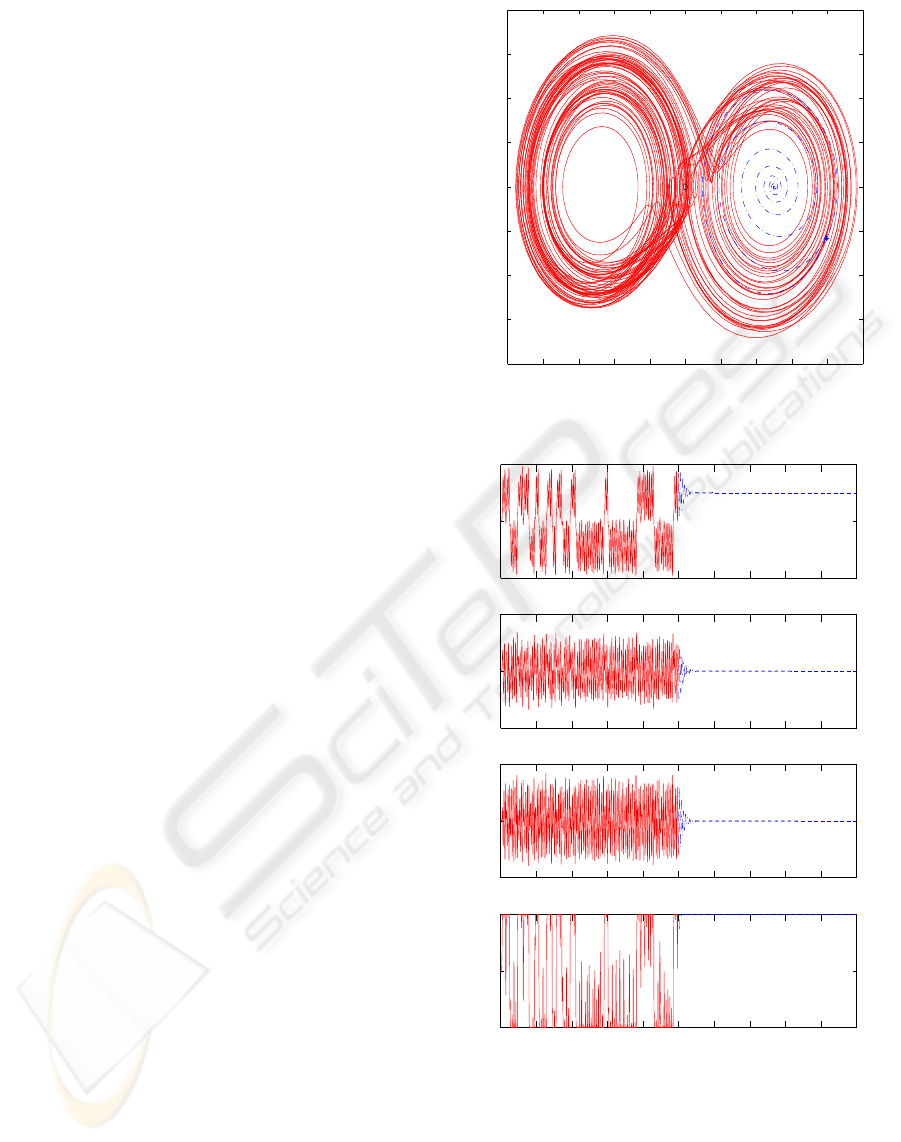
given in Fig. 1 - 3 : the phase-plane (i.e. x
1
versus
x
2
) trajectories are depicted in Fig. 1, the components
x
i
, i = 1, 2, 3 of the state-vector and the control input
are depicted in Fig. 2, and the adaptive gain K is de-
picted in Fig. 3. It is seen from these figures that the
chaotic behavior characterizing the system in open-
loop, is replaced by a stable trajectory at t ≥ 250sec
where the SAC is applied.
6 CONCLUSIONS
A class of stochastic Hopfield networks subject to
state-multiplicative noise where the network weights
jump according a Markov chain process have been
−1 −0.8 −0.6 −0.4 −0.2 0 0.2 0.4 0.6 0.8 1
−0.8
−0.6
−0.4
−0.2
0
0.2
0.4
0.6
0.8
x
1
x
2
Figure 1: Simulation Results.
0 100 200 300 400 500 600 700 800 900 1000
−1
0
1
x
1
0 100 200 300 400 500 600 700 800 900 1000
−1
0
1
x
2
0 100 200 300 400 500 600 700 800 900 1000
−1
0
1
x
3
Time [sec]
0 100 200 300 400 500 600 700 800 900 1000
−1
0
1
u
c
Time [sec]
Figure 2: Simulation Results.
considered. Stochastic passivity conditions for such
systems have been derived in terms of Linear Matrix
Inequalities. The results have been illustrated via sim-
plified adaptive control of a dynamic system which
exhibits a chaotic behavior when its is not controlled.
ICINCO 2008 - International Conference on Informatics in Control, Automation and Robotics
88

0 100 200 300 400 500 600 700 800 900 1000
−0.5
0
0.5
1
1.5
λ
1
Time [sec]
0 100 200 300 400 500 600 700 800 900 1000
−1
0
1
2
λ
2
Time [sec]
0 100 200 300 400 500 600 700 800 900 1000
−2
0
2
4
6
λ
3
Time [sec]
Figure 3: Simulation Results.
The control efficiency in stabilizing the chaotic pro-
cess has been demonstrated with simulations. The
results of this paper should encourage further study
of attempts to control chaotic systems with simplified
adaptive controllers.
REFERENCES
Boyd, S., El-Ghaoui, L., Feron, L., and Balakrishnan, V.
(1994). Linear matrix inequalities in system and con-
trol theory. SIAM.
Cabrera, J., Bormann, R., Eurich, C., Ohira, T., and Milton,
J. (2001). State-dependent noise and human balance
control. Fluctuation and Noise Letters, 4:L107–L118.
Cabrera, J. and Milton, J. (2004). Human stick balancing :
Tuning levy flights to improve balance control. Phys-
ical Review Letters, 14:691–698.
Dragan, V. and Morozan, T. (1999). Stability and robust
stabilization to linear stochastic systems described by
differential equations with markovian jumping and
multiplicative white noise. The Institute of Mathemat-
ics of the Romanian Academy, Preprint 17/1999.
Dragan, V. and Morozan, T. (2004). The linear quadratic
optimiziation problems for a class of linear stochastic
systems with multiplicative white noise and marko-
vian jumping. IEEE Transactions on Automat. Contr.,
49:665–675.
Fen, X., Loparo, K., Ji, Y., and Chizeck, H. (1992). Stochas-
tic stability properties of jump linear systems. IEEE
Transactions on Automat. Contr., 37:38–53.
Hu, S., Liao, X., and Mao, X. (2003). Stochastic hopfield
neural networks. Journal of Physics A:Mathematical
and General, 36:1–15.
Kaufman, H., Barkana, I., and Sobel, K. (1998). Direct
Adaptive Control Algorithms - Theory and Applica-
tions. Springer (New-York), 2 edition.
Kwok, H., Zhong, G., and Tang, W. (2003). Use of neurons
in chaos generation. In ICONS 2003, Portugal.
L¨ofberg, J. (2004a). YALMIP : A Toolbox for Modeling and
Optimization in MATLAB.
L¨ofberg, J. (2004b). YALMIP : A toolbox for modeling
and optimization in MATLAB. In Proceedings of the
CACSD Conference, Taipei, Taiwan.
Lure, A. and Postnikov, V. (1944). On the theory of sta-
bility of control systems. Applied Mathematics and
Mechanics (in Russian), 8(3):245–251.
Mazenc, F. and Niculescu, S.-I. (2001). Lyapunov stabil-
ity analysis for nonlinear delay system. Systems and
Control Letters, 42:245–251.
Poznyak, A. and Sanchez, W. Y. E. (1999). Identifica-
tion and control of unknown chaotic systems via dy-
namic neural networks. IEEE Transactions on Cir-
cuits and Systems E: Fundamental Theory and Appli-
cations, 46:1491–1495.
Stoica, A. and Yaesh, I. (2005). Hopfield networks with
jump markov parameters. WSEAS Transactions on
Systems, 4:301–307.
Stoica, A. and Yaesh, I. (2006). Delayed hopfield networks
with multiplicative noise and jump markov parame-
ters. In MTNS 2006, Kyoto.
X. Liao, G. C. and Sanchez, E. (2002). Lmi based approach
to asymptotically stability analysis of delayed neural
networks. IEEE Transactions on Circuits and Systems
E: Fundamental Theory and Applications, 49:1033–
1039.
Yaesh, I. and Shaked, U. (2005). Stochastic passivity and its
application in adaptive control. In CDC 2005, Kyoto.
PASSIVITY OF A CLASS OF HOPFIELD NETWORKS - Application to Chaos Control
89