
DESIGN OF AN ANALOG-DIGITAL PI CONTROLLER WITH
GAIN SCHEDULING FOR LASER TRACKER SYSTEMS
Christian Wachten, Lars Friedrich, Claas Müller, Holger Reinecke
Department of Microsystems Technology, University of Freiburg, Georges-Koehler-Allee 103, 79110 Freiburg, Germany
Christoph Ament
Institue for Automation and Systems Engineering, TU Ilmenau, 98693 Ilmenau, Germany
Keywords: Laser tracker system, PI controller with µC, Analog-digital design, Absolute distance measurement.
Abstract: Laser trackers are important devices in position metrology. A moving reflector is tracked by a laser beam to
determine its position in space. To ensure a proper function of the device the feedback control loop is an es-
sential part. An analog PI controller with online parameter adaptation and absolute distance measurement
ability is used to guarantee an optimal dynamic system. The feedback controller is connected to a quadrant
detector which serves as the sensor element in the control loop. The position of an incoming laser beam is
measured by the quadrant detector and the controller provides the input signals for a subsequent actuator.
The control variable is the deviation of the laser beam from the centre of the diode which should ideally be
zero. The actuator consists of two axes and each one is equipped with a rotatable mirror. The task of the
controller is to rotate the mirrors in such a way so that the laser beam follows the movements of the reflec-
tor. To design an optimal controller linear, time-invariant models of the actuator and the position sensor are
developed to optimize its parameters. The gain of the plant correlates with the distance between the reflector
and the laser tracker. To achieve the optimal dynamic performance the controller is automatically adapted to
the distance during operation. A method based on oscillation injection to measure the absolute distance is
developed. Due to higher dynamic demands a standard analog PI controller is implemented with the con-
troller gain tuned by digital potentiometers. A microcontroller is used to adjust the parameters and to esti-
mate the distance. During the power up sequence and in case of a beam loss the system is completely con-
trolled by the digital part.
1 INTRODUCTION
Laser trackers are devices which are used in position
metrology and in calibration tasks due to their capa-
bility of doing static as well as dynamic high accu-
racy measurements (Riemensperger & Gottwald
1990). A HeNe laser with a Gaussian beam profile
emits two light beams with different frequencies f
1
and f
2
. These beams are divided by an interferometer
into a reference beam and a measurement beam. The
measurement beam leaves the interferometer and is
deflected by the mirrors of an actuator in such a
manner that it follows the movement of a retrore-
flector. The reflected light is analyzed by a position
sensitive detector, the analog output signals of which
are used to determine the position of the incoming
beam. The reflected light beam also interferes with
the reference beam in the interferometer. So, by
measuring the two mirror angles of the actuator and
the relative distance given by the interferometer the
position of the reflector is calculated by using an
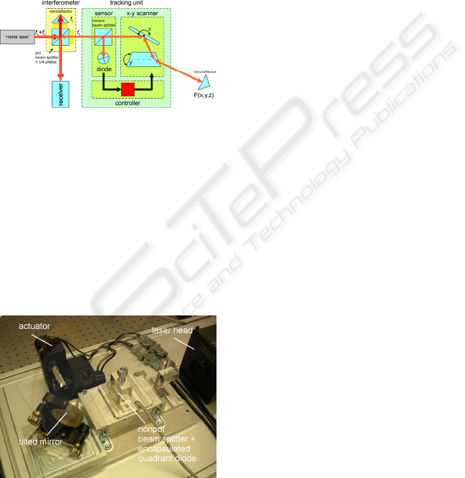
analytical model. Figure 1 shows the operation prin-
ciple.
An important part of the tracker is the feedback
controller in the tracking unit. It provides the input
signals for the actuator, so that the laser beam fol-
lows the movement of the retroreflector. The basic
task of the controller is to guarantee the proper inter-
ferometer function. Dynamic aspects like a high
velocity or high acceleration of the retroreflector
with a low contouring error are also important.
We present the development of a fast and cost ef-
fective analog feedback controller for a tracking unit
that can be used with laser tracker systems. The
5
Wachten C., Friedrich L., Müller C., Reinecke H. and Ament C. (2008).
DESIGN OF AN ANALOG-DIGITAL PI CONTROLLER WITH GAIN SCHEDULING FOR LASER TRACKER SYSTEMS.
In Proceedings of the Fifth International Conference on Informatics in Control, Automation and Robotics - SPSMC, pages 5-12
DOI: 10.5220/0001478600050012
Copyright
c
SciTePress
tracking unit is designed for working with an inter-
ferometer but can also act as an autonomous system
because of the integrated absolute distance meas-
urement technique. A distance of about eight meters
between the tracker unit and the reflector is easily
achieved in experiment without static tracking er-
rors. Furthermore, the lateral offset of the laser beam
does not exceed a quarter of the beam diameter and
thus guarantees stable interferometer functionality.
Figure 1: Operation principle of a laser tracker system.
The frequency f
1
represents the measurement beam and f
2
the reference beam.
2 SYSTEM COMPONENTS
The tracking unit consists of three components (see
figure 1). The first component is the sensor element
which is a combination of a nonpolarizing beam
splitter and a quadrant diode. The second component
is a x-y scanner with two magnetically driven mir-
rors that deflect the laser beam (galvanometer scan-
ner). The third component is the controller that con-
nects the sensor element with the actuator.
Figure 2: Photograph of the tracking unit. The two mirrors
of the actuator deflect the incoming laser beam. A tilted
mirror is used to adjust the light path.
The laser beam hits a nonpolarizing beam split-
ter. It has a division ratio of 50:50. Afterwards, it is
deflected by the scanner and is then reflected by the
retroreflector. The retroreflector has the unique
property that the incoming laser beam is reflected
into the same direction where it came from. On its
returning path the reflected beam hits the nonpolar-
izing beam splitter again and a part of the beam is
deflected on a quadrant diode. This diode provides
the analog input voltages for the feedback controller
since it has an integrated transimpedance amplifier.
The feedback controller generates the input signals
for the scanner. Ideally, the laser beam is centered
on the diode and the position signals equal zero
volts. By moving the reflector the laser beam leaves
the center on the diode and the position signals
change. The controller compensates the position
change and modifies the input signals of the actua-
tor. The two mirrors rotate and deflect the laser
beam in such a way that the offset becomes zero.
Figure 2 shows a photograph of the complete track-
ing unit.
2.1 Laser Head
The laser is a class II HeNe laser with a Gaussian
beam profile. It emits two linear, orthogonal polar-
ized beams with a split frequency of about 1.8 MHz.
The beam diameter is about 6 mm. The power P of
the laser is about 120 µW.
2.2 Magnetic Actuator
The magnetic actuator is a galvanometer scanner
produced by Cambridge Technology. It has silver
coated mirrors which allow a maximal beam aper-
ture of 10 mm. Each mirror is magnetically driven
and has its own analog PID controller to hold the
desired position. The transfer factor is 0.83 V/° (me-
chanical) at the input side of the controller and
0.5 V/° (mechanical) at the output side of the posi-
tion detector. Integrated sensors allow the measure-
ment of the rotation angle of the mirrors. The short
term stability is about 8 µrad. The maximal me-
chanical rotation angle is ± 12.5° limited by the used
assembly.
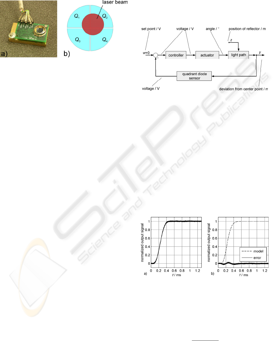
2.3 Quadrant Photodetector
The sensor element of the tracking unit is a quadrant
photodiode. Figure 3 shows a photograph of the pho-
todiode and a sketch of its quadrants. Each quadrant
is sensitive to light with a sensitivity that is specified
to 0.54 A/W at a wavelength of 900 nm. The spacing
ICINCO 2008 - International Conference on Informatics in Control, Automation and Robotics
6
between the quadrants is 0.2 mm, the quadrant ra-
dius is 3.99 mm.
Figure 3: Photograph of the quadrant detector a) and
sketch b) of its quadrants. The voltage level of the position
signals depends on the area that is covered by the laser
beam, its shape, its power and the wavelength.
The diode current depends on the power of the
laser beam, its shape, its wavelength and the area
that is covered. To perform a current to voltage
transformation a transimpedance amplifier is put on
the same circuit. The output of the amplifier consists
of three voltages that completely define the position
and the power of the laser beam. The signals can be
calculated with the following formulas:
4
4321
10)( ⋅+++= IIIIV
Sum
V/A (1)
4
4321
10))()(( ⋅+−+= IIIIV
TB
V/A (2)
4
4231
10))()(( ⋅+−+= IIIIV
LR
V/A (3)
The symbol I
i
represents the current of a quad-
rant Q
i
. The signal V
Sum
is the summation of the
voltages that are generated by each quadrant and
thus is an indicator for the total power of the incom-
ing light beam at a known wavelength. The signal
V
TB
, the so called top-bottom voltage, represents the
position of the laser beam in vertical direction. The
signal V
LR
, the so called left-right voltage, represents
the position of the laser beam in horizontal direction.
If for example the laser power is the same on each
quadrant, V
TB
and V
LR
become zero volts.
3 MODELING OF THE PLANT
A block diagram of the system is shown in fig-ure 4.
The output signal y of the system is the deviation of
the light beam from the center of the quadrant diode.
This deviation should become zero for each compo-
nent. The output signal y is a superposition of the
movement of the reflector and the compensation part
of the actuator. The gain between the mirror angle
and the movement of the light beam on the diode
depends on the distance between the reflector and
the tracking unit. This is modeled in the block “light
path”. The symbol z represents the position of the
reflector in space and thus is a three-dimensional
vector. The signal y represents the beam position on
the diode area and thus is a two-dimensional vector.
Figure 4: Block diagram of the plant. The different inputs
and outputs with their units are shown.
To design an optimal feedback controller, mod-
els are developed and the model parameters are
identified for the blocks “actuator”, “quadrant di-
ode” and “light path”.
3.1 Modeling of the Block “actuator”
To obtain a transfer function for the magnetic actua-
tor the step response is recorded for each axis moni-
toring the position output of the integrated angle
encoders. A square wave with a peak-peak voltage
of 100 mV (corresponding to an angle of about
0.06°) and a frequency of 30 Hz is applied to the
inputs of the scanner.
Figure 5: Normalized and averaged measurement a) of the
step response of the y mirror and the model b) of the step
response with its error. The step rises at t = 0 s.
Figure 5 shows the measured step response and
the step response of the model for the y mirror. It is
assumed that the scanner has PT
n
behavior and thus
can be modeled with a PT
n
element in (4).
i
n
i
i
i
sT
K
sH
)1(
)(
⋅+
=
, i = x,y (4)
DESIGN OF AN ANALOG-DIGITAL PI CONTROLLER WITH GAIN SCHEDULING FOR LASER TRACKER
SYSTEMS
7
The parameter K
i
describes the gain and the pa-
rameter T
i
represents the time constant for axis i.
The parameter n
i
stands for the order of the element.
To obtain the parameters the method of the time
percentage values is applied. Since the measurement
is not supposed to have ideal PT
n
behavior a least-
squares fit is done to optimize the parameters so that
the error between the model and the measurement
becomes minimal. The start parameters for the opti-
mization are the results given by the method of the
time percentage values (Schwarze 1962). The final
optimization yields in n
y
= 9 and T
y
= 27.51 µs for
the y mirror. The parameters for the x mirror result
in n
x
= 10 and T
x
= 23.42 µs. Taking into account
that the gain between the output signal and the me-
chanical deflection is 0.5 V/° the gains are calculated
to K
x
= 1.210 °/V and K
y
= 1.207 °/V, respectively.
The -3 dB frequency is about 1.8 kHz (model).
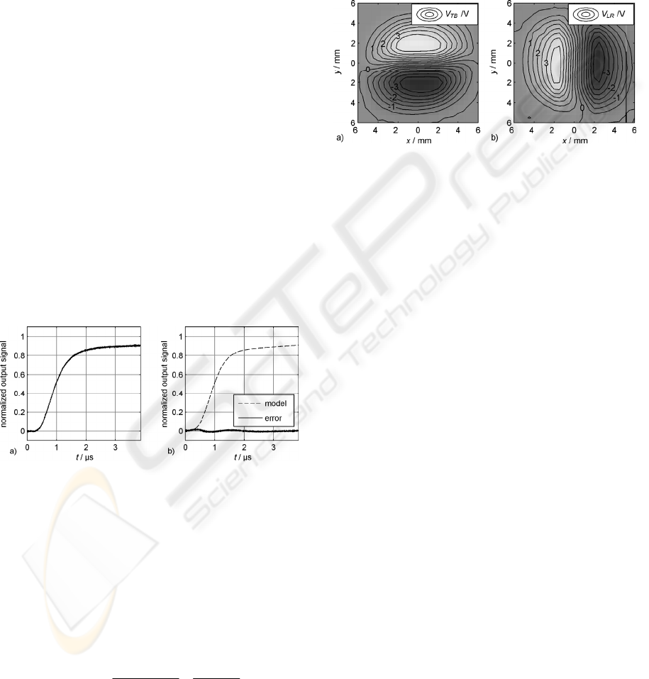
3.2 Modeling of the Block “diode”
The time response of the diode can be modeled in
the same way as the time response for the actuator.
A red LED is used to generate the step response be-
cause it is fast enough and its time response can be
neglected. The output signal V
Sum
is measured. The
LED has a power of about 7 µW. Figure 6 shows the
measurement and the model of the step response.
Figure 6: Normalized and averaged measurement a) of the
step response of the diode and the model b) with its error.
A red, pulsed LED is used to illuminate the active area.
The step rises at t = 0 s.
The modeling with only a single PT
n
element is
not applicable because there is a steep increase of
the signal until 1.6 µs. Afterwards, the signal in-
creases very slowly and does not reach 100% even
after 4 µs. Therefore, it can be shown that a good
approximation is a combination of a PT
n
element
and a PT
1
element. This is done in (5).
sT
g
sT
g
sH
D
n
D
⋅+
−
+
⋅+
=
2
1
1
1
)1(
)(
(5)
The parameters T
1
and T
2
represent time con-
stants of the two elements, the parameter g normal-
izes the output and the parameter n
D
represents the
order of the PT
n
element. All parameters are ob-
tained using a least squares fit so that the deviation
of the model and the measurement becomes mini-
mal. The optimal parameters are n
D
= 7, T
1
= 136 ns,
T
2
= 4.75 µs, g = 0.793. The model predicts a -3 dB
frequency of 250 kHz.
Figure 7: Local behavior of the diode. There is a nonlinear
relation between the output voltage and the position of the
beam.
Because the diode generates position signals not
only the time response is important but also its local
behavior. Figure 7 shows the local behavior of di-
ode. The quadrant diode was put onto an x-y station
and a laser diode with a power of 771 µW was in-
stalled in front of it. The station moves to 900 de-
fined positions that are placed in an equally spaced
square.
In figure 7 it can be seen that there is a nonlinear
relation between the position and the output volt-
ages. In the center of the diode the contour lines are
nearly parallel to the corresponding axis and so a
linearization is possible. It is obvious that the signal
V
TB
only depends on a movement in y direction and
V
LR
only depends on a movement in x direction. As a
result, each axis of the scanner can be regarded as
independent.
3.3 Modeling of the Block “light path”
The block “light path” depends on the position of the
reflector. If the angular errors are neglected the re-
flector can be approximated as its center point in a
plane (see figure 8a). The hitting point of the incom-
ing laser beam is point reflected with the center. An
offset between the incoming and the reflected laser
beam can have different reasons, for example a rota-
tion or a lateral displacement of the reflector.
ICINCO 2008 - International Conference on Informatics in Control, Automation and Robotics
8
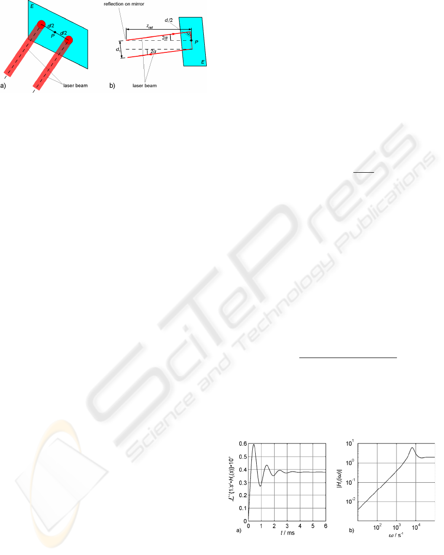
Figure 8: Modeling of the reflector. An incoming beam is
reflected at the center of the reflector.
The first effect is shown in figure 8b. The mirror
rotation angle is α. It is assumed that the reflector is
z
rad
away from the tracking unit. So the offset d
1
can
be written as
α
α
⋅⋅≈⋅⋅=
radrad
zzd 4)2sin(2
1
(6)
The second effect resulting in a beam offset is
the lateral displacement z
lat
of the reflector. The in-
dices represent the coordinate frame of the diode. So
it can be written as
ilati
zd
,,2
2 ⋅= , i = x,y (7)
The total deflection on the quadrant diode is a
combination of these two effects as shown in (8)
ii
ddy
,21
+= , i = x,y. (8)
4 CONTROLLER DESIGN
The controller has to be designed separately for the x
and the y-axis. Because of the decoupling of the
axes shown in figure 7 the problem is reduced to the
controller design for one axis. Exemplarily, the x-
axis is used to demonstrate the design process. It can
be derived from the block “light path” that the gain
of the plant correlates with the distance z
rad
. In a first
step it is assumed that z
rad
is constant. During opera-
tion the controller should be automatically adapted
to the distance so the restriction z
rad
= const. is
dropped. This adaptation to the distance is known as
gain scheduling.
The controller has to fulfill several requirements
for the use in laser tracker systems. First, the offset
of the beam should be smaller then a quarter of the
beam diameter to guarantee the interferometer func-
tion. Second, a high velocity of the reflector is nec-
essary to allow rapid movements of the object. The
third requirement is the robustness against vibrations
without any disturbance of the measurement accu-
racy. Of course, a large measurement volume is de-
sirable, too.
To achieve stationary accuracy the controller
should possess an integrating part because the plant
only consists of proportional blocks. A pure I con-
troller is also possible but a proportional part en-
hances the performance (Merz & Jaschek 1996). A
PI controller is well suited for plants with PT
n
be-
havior.
A standard PI controller is proposed due to its
simple design and to reduce the analog circuit com-
plexity because the derivative part is missing. The
transfer function is well known and given in (9).
⎟
⎟
⎠
⎞
⎜
⎜
⎝
⎛
⋅
+⋅=
sT
KsH
R
RR
1
1)(
(9)
The parameter K
R
describes the gain of the con-
troller and T
R
its time constant. First, these parame-
ters are determined by the classic frequency re-
sponse method as described by Föllinger (1994).
The time constant T
R
is set to T
x
= 23.42 µs because
this is the dominating time constant of the x mirror
in the plant. The gain K
R,30°
is set to 0.1231 to obtain
a phase margin of 30° for the gain crossover fre-
quency. It is of interest to examine the disturbance
transfer function because the set point (w(t) = 0) is
constant. H
z
(s) is calculated in (10) and is derived
from the block diagram in figure 4.
)()()(1
2
)(
sHsHsH
sH
DRS
z
⋅⋅+
=
(10)
To estimate the performance of the classic feed-
back controller the response to a ramp in z
lat,i
and the
magnification factor is simulated for the disturbance
transfer function in (10).
Figure 9: Simulation of the ramp response a) and the fre-
quency response b) of the disturbance transfer function
with a classic PI controller.
A ramp is chosen because it is the strongest re-
quirement concerning the reflector movement. A
DESIGN OF AN ANALOG-DIGITAL PI CONTROLLER WITH GAIN SCHEDULING FOR LASER TRACKER
SYSTEMS
9
step is not applicable because in reality the position
of the retroreflector cannot rapidly change.
Figure 9a) shows the response on a ramp in z
lat
(t)
at the output y
x
of the system. The maximal value of
the overshoot at the output y
x
is 0.60·10
-3
m until a
constant contouring error of 0.38·10
-3
m is reached.
Figure 9b) shows the frequency response. Low fre-
quencies are damped due to the integrating part. But
there is a magnification factor of 6.3 at a frequency
of 1 kHz.
The maximal value is reached at the overshoot,
but the contouring error is much lower. Therefore,
the maximum of the ramp response has to be mini-
mized so that the overshoot is reduced at the cost of
the contouring error. The aim is the adaptation of the
overshoot to the contouring error. For ω→∞,
|H
z
(iω)| converges to 2, so an arbitrary factor of 4 is
proposed for all frequencies to guarantee robustness
against vibrations. To identify the optimal controller
parameters K
R
and T
R
were varied in a range of
K
R
= 0.1·K
R,30°
…10·K
R,30°
and T
R
= 0.1·T
x
…10·T
x
.
The raster was ΔK
R
= 0.05·K
R,30°
and ΔT
R
= 0.05·T
x
.
Figure 10 shows the ramp response and frequency
response for the optimized parameters K
R,opt
= 0.542
and T
R,opt
= 135 µs. The maximal value of the re-
sponse is about 0.51·10
-3
m with a very low over-
shoot and the magnification factor does not exceed
4. So, the quality of control is much better in com-
parison with the classic approach.
Figure 10: Simulation of the ramp response a) and the
frequency response b) of the disturbance transfer function
with optimal controller parameters in regard to contouring
error and magnification factor.
It was assumed that the total gain is focused in
the parameter K
R
. This is not the case in a real sys-
tem. The real total gain is a product of the controller
gain, the mirror gain, the light path and the sensitiv-
ity of the quadrant diode. It can be written as
DradxRoptR
KzKKK ⋅⋅⋅⋅= 4
,
(11)
Dradx
optR
R
KzK
K
K
⋅⋅⋅
=⇔
4
,
(12)
To adapt the controller gain, the parameters K
R
and K
D
have to be updated during operation (gain
scheduling). The parameter K
D
is obtained by meas-
uring the voltage V
Sum
of the quadrant diode. The
parameter z
rad
has to be estimated.
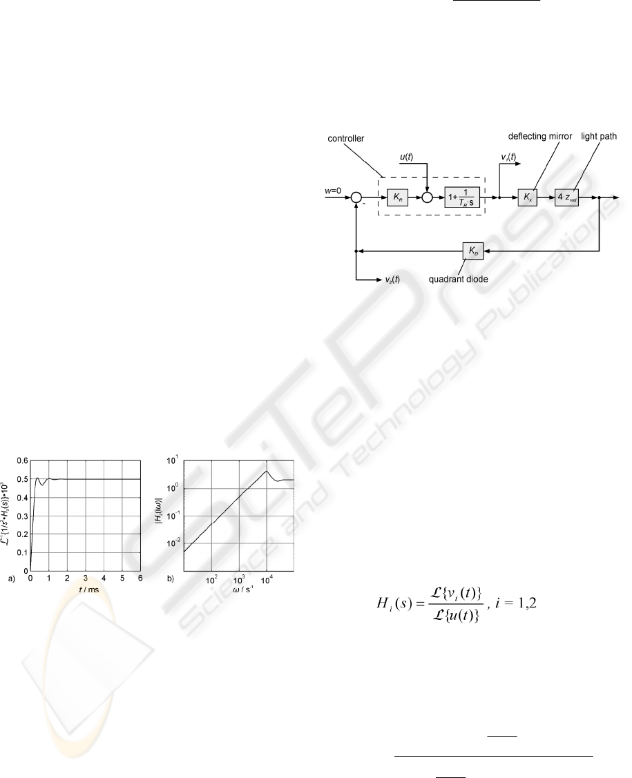
Figure 11: Control loop with introduced signal u(t) to es-
timate z
rad
. The signals v
1
(t) and v
2
(t) can be measured and
depend on z
rad
.
To estimate z
rad
a known signal u(t) is introduced
into the control loop (figure 11). Only the spectral
components are considered which are below the cut-
off frequency of the diode. So, it is possible to sim-
plify the transfer functions and consider only their
proportional parts. But the time response of the con-
troller cannot be neglected because there is a strong
dependency on low frequencies introduced by the
integrating part. The multiplication with z
rad
is mod-
eled as proportional part because z
rad
changes slowly
in comparison to the system dynamic.
The signals v
1
(t) and v
2
(t) depend on the distance
z
rad
. The transfer functions can be calculated with
(13).
(13)
It can be shown that there is a higher sensitivity
of
|)(|
01
ω
iH to a change in z
rad
if signal v
1
(t) is
measured. With (13) and figure 11 the transfer func-
tion H
1
(s) is calculated in (14).
xradDR
R
R
KzKK
sT
sT
sH
⋅⋅⋅⋅⋅
⎟
⎟
⎠
⎞
⎜
⎜
⎝
⎛
⋅
++
⋅
+
=
4
1
11
1
1
)(
1
(14)
The signal v
1
(t) is a superposition of the movement
of the reflector and the introduced signal u(t). A si-
ICINCO 2008 - International Conference on Informatics in Control, Automation and Robotics
10

nusoidal signal with a frequency ω
0
is proposed. So,
a subsequent band-pass filter with the center fre-
quency ω
0
suppresses the disturbance signal intro-
duced by the reflector. To estimate the distance z
rad
the amplitude of u(t) is compared with the amplitude
v
1
(t) and so |H
1
(iω)| is calculated. With the experi-
mentally obtained relationship for K
D
in (15), z
rad
is
calculated in (16). The proportional value m has a
value of 45.13 V
-1
m
-1
.
x
Sum
D
K
Vm
K
⋅
⋅
=
4
(15)
(
))2(1(
4
0
42
0
222
ωω
RRrad
TTAAz +−−= (16)
)
(
)
)1(/
2
0
222
0
22
ωω
RSumRR
TmVKATA +−
with
|)(|
01
ω
iHA = .
To obtain an appropriate value for the amplitude
of the signal u(t) the beam deviation y
x
(t) from the
center of the quadrant diode is analyzed. The devia-
tion should be smaller than a quarter of the beam
diameter to guarantee the interferometer function.
During distance estimation the deviation y
x
(t) is a
superposition of the lateral movement of the reflec-
tor z
lat,x
(t) and the introduced signal u(t). Therefore,
the amplitude of the signal u(t) is chosen to be only
10% of the maximal deflection so that the maximal
velocity v
lat
is not reduced. With the transfer func-
tion H
2
(s) and a maximal amplitude y
x,max
of y
x
(t) the
amplitude u
0
is calculated in (17).
|)(|
02
max,0
ω
iH
K
yu
D
x
⋅=
(17)
Because z
rad
is located in the denominator of (17)
its increase leads to a decreasing amplitude u
0
. Ac-
cording to the described limit of 10%, y
x,max
is set to
R/20 with R being the radius of the beam.
5 PRACTICAL
CONSIDERATIONS
The feedback controller is implemented in an analog
design. To generate the signal u(t), to measure the
signal v
1
(t) and to adapt the gain of the controller, a
microcontroller is used. The microcontroller is an
ATmega128 and is programmed in C. The variable
gain control is realized by digital potentiometers that
are set by the microcontroller. Figure 12 shows the
used circuit for one axis. The digital potentiometer
R
2
offers 127 linearly arranged steps. The resistance
can be adjusted between 1 kΩ and 50 kΩ.
The analog PI controller is built with standard
components without complex serial or parallel circi-
uts resulting in a time constant of T
R
= 132 µs and a
adjustable gain between K
R
= 6.00·10
-3
… 300·10
-3
.
The parameter T
R
remains constant even if the po-
tentiometers change their value. Because of the dis-
crete potentiometer positions there is an error be-
tween the optimal controller gain and the achieved
controller gain. There are only integer positions n
int
available. To obtain an optimal value for K
R
the
theoretical real number n
real
for the potentiometer
position is calculated. Afterwards, n
real
is rounded
down and up and the lower and the upper controller
gains K
l
and K
u
are calculated. The controller gain
with the minimal error in regard to the optimal value
is chosen.
Figure 12: Microcontroller controlling a digital potenti-
ometer and analog PI controller exemplarily shown for the
x-axis.
After power up sequence and beam loss during
operation, the laser beam searches the reflector in a
defined area. This is done by deflecting the mirrors
of the actuator without opening the feedback loop.
The influence of the analog part is reduced and only
the digital part controls the mirror deflection.
Figure 13 shows the operation principle. The
digital potentiometer is set to its maximal value. So,
the influence of the sensor signal to the input of the
PI controller is weak. This is comparable to an open-
ing of the feedback loop and the signal can be cross
talked easily.
The microcontroller introduces a signal at the in-
put of the PI controller. At the same time the re-
duced sensor signal of the diode acts as a distur-
bance variable. The output of the controller is digi-
talized and is compared to the set up variable w
α
.
The microcontroller multiplies the gain K
µ
with the
deviation e. So, the plant with integrating behavior is
controlled via a P controller which is a good combi-
DESIGN OF AN ANALOG-DIGITAL PI CONTROLLER WITH GAIN SCHEDULING FOR LASER TRACKER
SYSTEMS
11
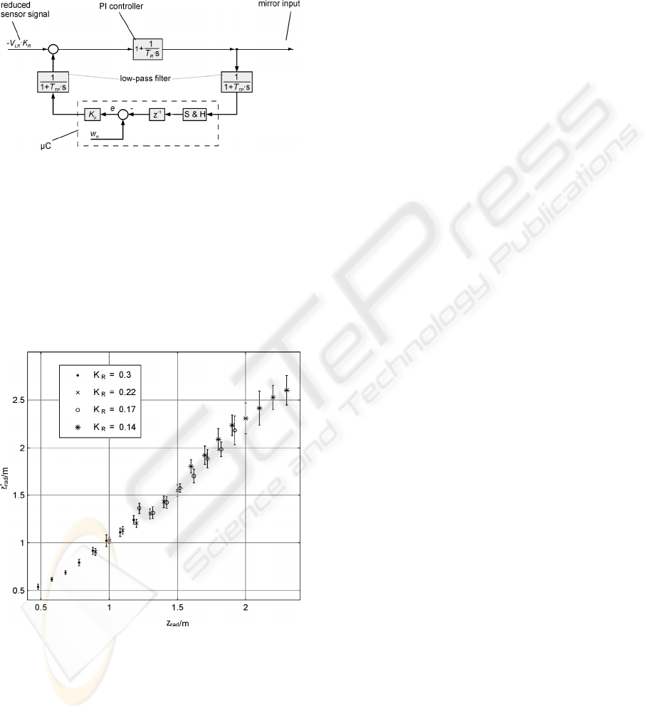
nation (Merz & Jaschek 1996). The DA conversion
at the output of the microcontroller is done via a
pulse width modulation (PWM) with a frequency of
14.4 kHz and a low-pass filter with a cut-off fre-
quency of 300 Hz (smoothing function).
Figure 13: Operation principle for deflecting the mirrors in
a defined way.
The output of the controller is digitized by the in-
tegrated AD converter of the microcontroller. To
reduce alias effects a low-pass filter with a cut-off
frequency of 300 Hz is used, too.
K
µ
represents the total gain of the control loop
and is set to K
µ
= 41. This is a tenth of the value of
the stability limit. So, the safety margin is high
enough to avoid instability.
Figure 14: Estimated z’
rad
as a function of the real z
rad
.
Each point is averaged 20 times with its two-time standard
deviation. To increase readability the measurements for
K
R
= 0.3 show a horizontal offset of -0.02 m and for
K
R
= 0.17 an offset of +0.02 m.
To estimate the distance z
rad
between the system
and the retroreflector a signal is introduced in the x-
axis (figure 11). To reduce the computing and pro-
gramming complexity a square wave with a fre-
quency of 200 Hz instead of a sinusoidal signal is
used. An analog band pass filter with the same fre-
quency is used for signal pre-processing. Only the
basic frequency is considered in the signal analysis.
Because the movement of the retroreflector has only
few spectral components in the pass-band the gain
can be increased without leaving the input range of
the AD converter. So, a small value of u
0
is suffi-
cient to detect the amplitude of v
1
(t) with a DTFT.
Figure 14 shows the distance estimation for dif-
ferent gains of the controller. To reduce the time
effort only distances between 0.5 m and 2.3 m are
measured. The estimated value shows a good accor-
dance to the real values. The variance increases with
the distance because of the reduced sensitivity of the
measured voltage to the distance.
Further experiments have shown that the retrore-
flector can be moved with a maximal velocity of
v
max
= 2.5 m/s at unlimited acceleration and a beam
offset of a quarter of the beam diameter. Distances
between 0.5 m and 7.8 m (length of laboratory) were
tested without tracking problems.
6 CONCLUSIONS
An analog PI controller with additional features was
presented for the use in laser tracker systems. It is
fast to detect a rapid beam movement and shows
good control accuracy. Functions as gain scheduling
and distance estimation are integrated in this hybrid
design consisting of a digital and analog part.
REFERENCES
Föllinger, O., 1994. Regelungstechnik. 8
th
ed. Heidelberg:
Hüthig GmbH.
Merz, L. & Jaschek, H., 1996. Grundkurs der
Regelungstechnik. 13
th
ed. München/Wien: R.
Oldenburg Verlag.
Riemensperger, M. & Gottwald, R., 1990. Kern Smart 310
– Leica’s Approach to High Precision 3D Coordinate
Determination, In: F. Löffler, 2
nd
International Work-
shop on Accelerator Alignment. Hamburg, Germany,
10-12 September 1990. pp. 183-200.
Schwarze, G., 1962. Bestimmung der
regelungstechnischen Kennwerte von P-Gliedern aus
der Übertragungsfunktion ohne
Wendetangentenkonstruktion, Messen, Steuern,
Regeln, 5, pp. 447-449.
ICINCO 2008 - International Conference on Informatics in Control, Automation and Robotics
12
