
SHOE GRINDING CELL USING VIRTUAL MECHANISM
APPROACH
Bojan Nemec and Leon Zlajpah
Jozef Stefan Institute, Jamova 39, 1000 Ljubljana, Slovenia
Keywords:
Robotics, Redundant robot control, Force control, Shoe grinding.
Abstract:
The paper describes the automation of the shoe grinding process using an industrial robot. One of the major
problems of flexible automation using industrial robots is how to avoid joint limitations, singular configuration
and obstacles. This problem can be solved using kinematically redundant robots. Due to the circular shape of
the grinding disc, the robot becomes kinematically redundant. This task redundancy was efficiently handled
using virtual mechanism approach, where the tool is described as a serial mechanism.
1 INTRODUCTION
Shoe production is most likely labor intensive; the
rate of automation is usually low. Therefore it is con-
sidered as the industry suitable for the counties with
low labor cost (Taylor and Taylor, 1988; Nemec and
et all, 2003). In last years new aspect in shoe pro-
duction is arising - custom made shoes (Dulio and
Boer, 2004). The customization in mass shoe pro-
duction requires complex information system and full
automation of planning, production and distribution
processes. One of the major challenges is how to gen-
erate robot trajectories base solely on the CAD model
of the shoe. Manual teaching and trajectory test-
ing phases are not acceptable for customized shoes,
where virtually each work-piece on the production
line can differ from the previous one. Therefore, we
haveto design tools which enable to generate fault tol-
erant robot trajectories. This is usually accomplished
using complex task planning algorithms, which are in
most cases off-line batch procedures. In (Nemec and
Zlajpah, 2008) we proposed a solution based on con-
trol algorithms for the kinematicaly redundant robot,
where we sacrificed exact orientation of the tool in
order to achieve additional degrees of redundancy. In
this paper, we propose a new approach, called virtual
mechanism approach. The proposed algorithm was
applied to the shoe grinding cell, which uses an in-
dustrial robot with 7 D.O.F.
2 SOLVING TASK KINEMATIC
REDUNDANCY USING
VIRTUAL MECHANISM
APPROACH
Robotic systems under study are n degrees of free-
dom (DOF) serial manipulators. We consider redun-
dant systems, which have more DOF than needed to
accomplish the task, i.e. the dimension of the joint
space n exceeds the dimension of the task space m,
n > m and r = n − m denote the degree of the re-
dundancy. Let the configuration of the manipulator
be represented by the a vector q
q
q
r
of n joint positions,
and the end-effector position (and orientation) by m-
dimensional vector x
x
x
r
of the robot tool center point
positions (and orientations). The relation between the
joints and the task velocities is given by the following
well known expression
˙
x
x
x
r
= J
r
˙
q
q
q
r
(1)
where J
r
is the m×n manipulator Jacobian matrix.
The solution of the above equation for
˙
q
q
q
r
can be given
as a sum of the particular and the homogeneous solu-
tion
˙
q
q
q
r
=
¯
J
r
˙
x
x
x
r
+ N
r
ξ (2)
where
¯
J
r
= W
−1
J
T
r
(J
r
W
−1
J
T
r
)
−1
. (3)
Here,
¯
J
r
is the weighted generalized-inverse of J
r
, W
is the weighting matrix, N
r
= (I−
¯
J
r
J
r
) is a n×n ma-
trix representing the projection into the null space of
J
r
, and ξ is an arbitrary n dimensional vector. We will
denote this solution as the generalized inverse based
159
Nemec B. and Zlajpah L. (2008).
SHOE GRINDING CELL USING VIRTUAL MECHANISM APPROACH.
In Proceedings of the Fifth International Conference on Informatics in Control, Automation and Robotics - RA, pages 159-164
DOI: 10.5220/0001480901590164
Copyright
c
SciTePress
redundancy resolution at the velocity level (Nenchev,
1989). The homogenous part of the solution belongs
to the Jacobian null-space. Therefore, we will denote
it as
˙
q
q
q
n
,
˙
q
q
q
n
= N
r
ξ . Now consider the case where
the robot Jacobian matrix J
r
is defined in Cartesian
(world) coordinate system and the dimension of the
Jacobian is 6×n, but the task is described in another
coordinate system. It can be shown that the transfor-
mation from the Cartesian to the task space can be
very complex. As an alternative approach we propose
to model the tool as a serial kinematic link. Let con-
sider the general case where the robot holds the object
to be machined and the work tool is fixed, as illus-
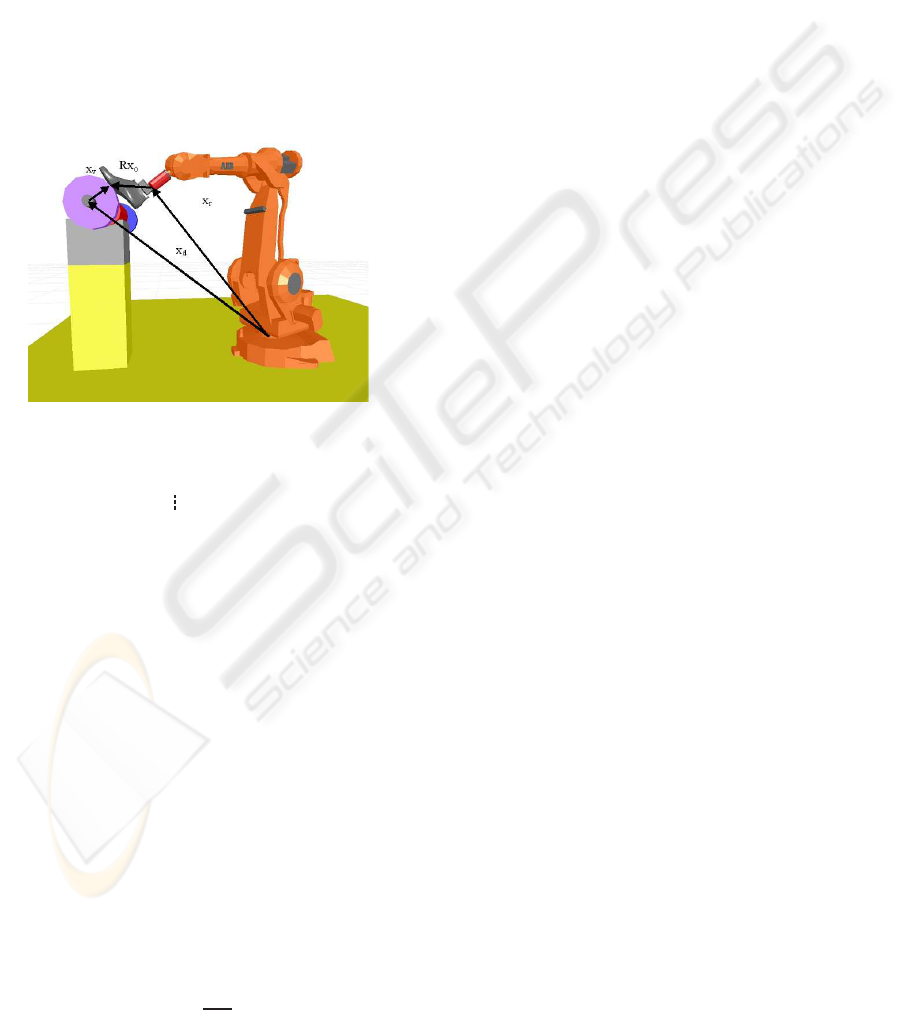
trated in Fig. 1. In such a case, we can define the
direct kinematic transformation as
Figure 1: The robot holds the object and the work toll is
fixed.
x
x
x
r
+
R I
x
x
x
o
= x
x
x
d
+ x
x
x
v
(4)
where x
x
x
r
is the robot Cartesian position and orienta-
tions, R is the robot tool rotation 3× 3 dimensional
matrix, x
x
x
o
is the 6 × 1 vector of the object position
and orientation, x
x
x
v
is the 6 × 1 vector of position and
orientation of the top of the virtual mechanism and
6× 1 vector x
x
x
d
describes the distance and orientation
between the base coordinates system and the work
tool coordinate system. Let consider robot and virtual
mechanism as one mechanism with n+ n
v
degrees of
freedom. The configuration of the virtual mechanism
can be described with the n
v
× 1 dimensional vector
q
q
q
v
. The new task position is
x
x
x = x
x
x
r
− x
x
x
v
(5)
and the Jacobian of this new mechanism can be ex-
pressed as
J = [J
r
| − J
v
] (6)
where the Jacobian of the virtual mechanism J
v
is de-
fined as
J
v
=
∂x
x
x
v
∂q
q
q
v
. (7)
As we can see, the task space preserves it’s dimen-
sion, while the joint space is increased with the di-
mension of the virtual mechanism. This approach has
two major advantages. First, we can use the existing
robot Jacobian, which is assumed to be known. Sec-
ond, the augmented part of the Jacobian has very sim-
ple structure in most cases. Note that Eq. 4 does not
handle orientations correctly, since orientation vec-
tors can not be simply added in general case. There-
fore, using Eq. 4 and 5 we obtain an approximate so-
lution regarding the orientation vector. In most cases,
the difference between the desired and the real orien-
tation vector is small and is acceptable for operations
like brushing and polishing. If orientations are impor-
tant, we can use equation 4 and 5 for the calculation
of positions only, while the orientations have to be
calculated using rotation matrices as follows.
R
o
= R
v
T
R (8)
Here, R
o
and R
v
are 3×3 rotation matrices describing
object rotation against virtual mechanism and virtual
mechanism rotation expressed in the robot base co-
ordinate system. The corresponding orientation vec-
tor can be than obtained using the transformation of
the rotation matrix to the orientation vector described
with euler or roll pitch yaw notation. Note that using
this ’correct’ transformation also rotation part of the
Jacobian described by Eq. 6 becomes more complex.
On the other hand, when the Jacobian is used in the
control loop, only approximate values of Jacobian are
needed. Therefore, control algorithm based on Jaco-
bian defined by Eq. 6 gives equal results as control
algorithm using the Jacobian calculated from rotation
matrices, as described with Eq. 8.
3 CONTROL
Using the virtual mechanism approach, we can di-
rectly apply any control algorithm for the kinemati-
cally redundant robot. A suitable choice is the con-
trol law using generalized inverse-based redundancy
resolution at velocity level in the extended opera-
tional space. Redundancy resolution at the velocity
level is favorable because it enables direct implemen-
tation of the gradient optimization scheme for the sec-
ondary task. The gradient projection technique has
been widely used for the calculation of the null space
velocity that optimizes the given criteria. The rea-
son for this is that a variety of performance criteria
can be easily expressed as gradient function of joint
coordinates. Although the control law using general-
ized inverse-based redundancy resolution at velocity
level can not completely decouple the task and the
ICINCO 2008 - International Conference on Informatics in Control, Automation and Robotics
160
null space (Oh et al., 1998; Park et al., 2002; Ne-
mec and Zlajpah, 2000; Nemec and Zlajpah, 2001),
it enables good performance in real implementation
(Nemec et al., 2007). The joint space control law is
τ
c
= HJ
T
(
¨
x
x
x
d
+ K
v
˙
e
e
e
x
+ K
p
e
e
e
x
+ K
f
e
e
e
f
−
˙
J
˙
q
q
q) +
HN(
¨
q
q
q
nd
+ K
n
˙
e
e
e
n
−
˙
N
˙
q
q
q) + h
h
h+ J
T
f
f
f (9)
where J is the Jacobian matrix, H is n× n inertia ma-
trix, h
h
h is n-dimensional vector of the centrifugal, cori-
olis and gravity forces, f
f
f is n-dimensional vector of
the external forces acting on the manipulator’s end ef-
fector and K
p
, K
v
, K
f
and K
n
are diagonal matrices
representing positional, velocity, force and null-space
feedback gains. The first term of the control law cor-
responds to the task-space control torque τ
x
, the sec-
ond to the null-space control torque τ
n
and the third
and the fourth is used to compensate the non-linear
system dynamics and the external force, respectively.
Here, e
e
e
x
= x
x
x
d
− x
x
x are the task-space tracking error,
e
e
e
f
= f
f
f
d
− f
f
f and
˙
e
e
e
n
=
˙
q
q
q
nd
−
˙
q
q
q
n
is the null-space track-
ing error. x
x
x
d
, f
f
f
d
and
˙
q
q
q
nd
are the desired task coordi-
nates, desired force and the desired null space veloc-
ity, respectively. The details of the control law deriva-
tion can be found in (Nemec and Zlajpah, 2000; Ne-
mec et al., 2007).
An attention should be paid on the selection of the
inertia of the virtual link. The inertia matrix H has the
form
H =
H
r
0
0 H
v
(10)
where H
r
is the robot inertia matrix and H
v
is the di-
agonal matrix describing the virtual mechanism iner-
tia. Clearly, H
v
can not be zero, but arbitrary small
values can be chosen describing the lightweight vir-
tual mechanism. Selection of the inertia matrix of the
virtual mechanism affects only the null space behav-
ior of the whole system. Heavy virtual links with high
inertia would slow down the movements of the virtual
links. Therefore, low inertia of virtual links is an ap-
propriate choice. On the contrary, we can assume that
no gravity, coriolis and centrifugal forces act on the
virtual links and the corresponding terms in the vector
h
h
h can be set to zero. Control law 9 assumes feedback
from all joints, including non-existing virtual joints.
There are multiple choices how to provide the joint
coordinates and the joint velocities of the virtual link.
A suitable method is to build a simple model com-
posed of a double integrator
˙
q
q
q
v
=
Z
H
−1
v
τ
cv
(11)
q
q
q
v
=
Z
˙
q
q
q
v
where τ
cv
is the part of the control signals correspond-
ing to the virtual link.
4 MOTION OPTIMIZATION
As we mentioned previously, one of the main prob-
lems in automatic trajectory generation is the inabil-
ity to assure that the generated trajectory is feasible
using a particular robot, either because of possible
collisions with the environment or because of the lim-
ited workspace of the particular robot. Limitations in
the workspace are usually not subjected to the tool
position, but rather to the tool orientation. Another
sever problem are wrist singularities, which can not
be predicted in the trajectory design phase on a CAD
system. A widely used solution in such cases is off-
line programming with graphical simulation, where
such situation can be detected in the design phase
of the trajectory. Unfortunately this is a tedious and
time consuming process and therefore not applicable
in customized production, where almost each work
piece can vary from the previous one (Dulio and Boer,
2004; Nemec and Zlajpah, 2008). The problem can be
efficiently solved using the null space motion, which
changes the robot configuration, but does not affect
the task space motion. The force and the position
tracking are of the highest priority for a force con-
trolled robot and are therefore considered as the pri-
mary task. The secondary task is defined by the opti-
mization of a given cost function.
Let p be the desired cost function, which has to be
maximized or minimized. Then the velocities
˙
q
q
q
n
= kNH
−1
(
δp
δq
1
,
δp
δq
2
, .....
δp
δq
n
, ) (12)
in Eq 12 maximize cost function for any k > 0 and
minimize cost function for any k < 0 (Asada and Slo-
tine, 1986), where k is an arbitrary scalar which de-
fines the optimization step. In our case we have se-
lected a compound p which maximizes the distances
between obstacle and the robot links or robot work
object, maximizes the distance to the singular con-
figuration of the robot and maximizes the distance in
joint coordinates between current joint angle and joint
angle limit. We define the cost function as a sum
of three cost functions p = p
a
+ p
l
+ p
s
, where p
a
denotes cost function for obstacle avoidance, p
l
cost
function for avoiding joint limits and p
s
cost function
for singularity avoidance. We select the cost func-
tion for obstacle avoidance as (Khatib, 1986; Khatib,
1987) p
a
=
1
2
Ed
2
0
, where E is an l × l rotation matrix
describing the direction of an artificial potential field
pointing from the obstacle, l is the dimension of the
position sub-space and d
0
is the shortest distance be-
tween the obstacle and the robot body. In our case the
desired objective is fulfilled if the imaginary force is
applied only on the robot joints. The cost function for
the joint limits avoidance is defined as (Nemec and
SHOE GRINDING CELL USING VIRTUAL MECHANISM APPROACH
161
Zlajpah, 2008; Chaumette and Marchand, 2001)
p
l
=
(q
max
− q)
2
, |q
max
− q)
2
| < ε
0
(q
min
− q)
2
, |q
min
− q)
2
| < ε
(13)
where ε is a positive constant defining the neighbor-
hood of joint limits. For the singularity avoidance
we use the manipulability index defined as(Asada and
Slotine, 1986)
p
s
=
q
|JJ
T
| (14)
Then, the desired null space velocity for our task are
calculated using
˙
q
q
q
n
= NH
−1
(k
a
J
03
Vd − 2k
l
(q
q
q
l
− q
q
q) − 2k
s
δJ
δq
q
q
J
T
(15)
Matrix J
03
is the Jacobian matrix calculated from the
robot base to the robot wrist. Scalars k
a
, k
l
and k
s
are
appropriate positive constants defining the optimiza-
tion step. In real implementation, k
a
and k
l
are set to
zero if the observed point is away enough from the
possible collision points and joints are far away from
their limits, respectively. Similar, the last term of
˙
q
q
q
n
is not computed if the manipulability index is large
enough. Unfortunately, the partial derivative
δJ
δq
q
q
is not
easy to calculate. However, we can use the numerical
derivative of the manipulability measure p
s
instead.
Vector q
l
denotes the physical joint limit in the range
[q
min
, q
max
].
5 SHOE GRINDING
In the shoe assembly process, in order to attach the
upper with the corresponding sole, it is necessary to
remove a thin layer of the material off the upper sur-
face so that the glue can penetrate the leather. To
do this, the robot has to press the shoe against the
grinding disc with the desired force while executing
the desired trajectory. In the past, there were sev-
eral approaches how to automate this operation. For
mass production, there are special NC machines avail-
able. Their main drawback is relatively complicated
setup and are therefore not suitable for the custom
made shoes. Required flexibility is offered by the
robot based grinding cell. In the EUROShoeE project
(Dulio and Boer, 2004), a special force controlled
grinding head has been designed. The robot manipu-
lated with the grinding head while the shoe remained
fixed on the conveyor belt (Jatta et al., 2004). The
main drawback of this approach is relatively heavy
and expensive grinding head. Additionally,force con-
trol can be applied only in one direction. In our ap-
proach, the robot holds the shoe and presses it against
the grinding disc of a standard grinding machine as
used in the shoe production industry. The impedance
force control was accomplished by the robot using
universal force-torque sensor mounted between the
robot wrist and the gripper which holds the shoe last.
It is well known that the kinematic redundancy en-
ables greater flexibility in execution of complex tra-
jectories. For example, also humanoid hand dex-
terity is subjected by it’s is kinematical redundancy.
We used Mitsubishi Pa10 robot with 7 D.O.F in our
roughing cell, which has one degree of redundancy.
Additional two degrees of redundancy were obtained
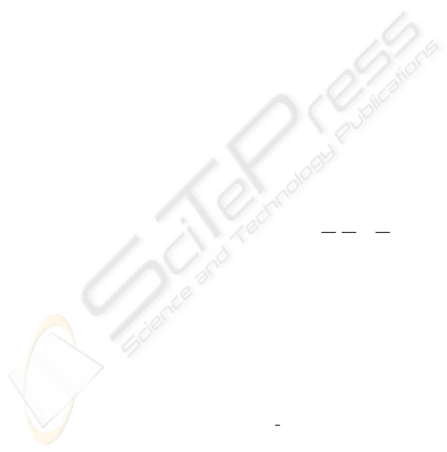
by treating the grinding disc as a virtual mechanism.
The surface of the grinding disc can be naturally de-
scribed with the outer surface of the torus, where R
and r are the corresponding radius of the grinding
disc, as shown in the Fig. 2. Let x be the task (Carte-
sian) coordinate of the whole system. Assuming that
the robot tool position and robot Jacobian is known,
the forward kinematics can be easily expressed as
j
R
r
z
y
γ
Figure 2: Rotary brush presented as torus.
x
x
x = x
x
x
r
+
s
ϕ
(R+ rc
γ
)
rs
ψ
c
ϕ
(R+ rc
γ
)
0
−ϕ
ψ
, (16)
while the corresponding Jacobian is
J =
J
r
c
ϕ
(R+ rc
ψ
) −s
ϕ
rs
γ
0 rc
ψ
−s
ϕ
(R+ rc
ψ
) − c
ϕ
rs
γ
0 0
−1
0 1
. (17)
Here, we used the abbreviation c
ϕ
= cos(ϕ), c
γ
=
cos(γ), s
ϕ
= sin(ϕ) and s
γ
= sin(γ). Thus we have 9
degrees of freedom, 6 of them are required to describe
the grinding task, while the remaining three degrees
of freedom are used for the obstacle avoidance, joint
limits avoidance and singularity avoidance.
ICINCO 2008 - International Conference on Informatics in Control, Automation and Robotics
162
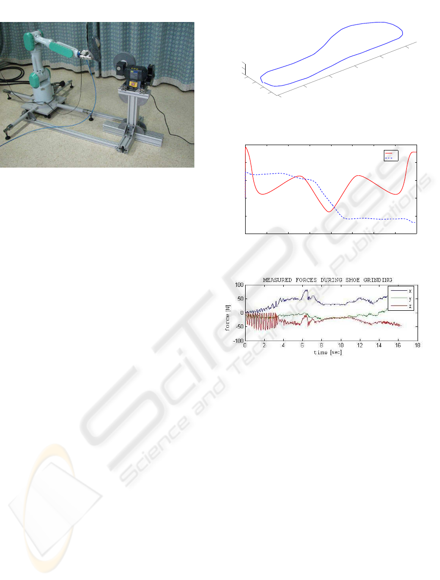
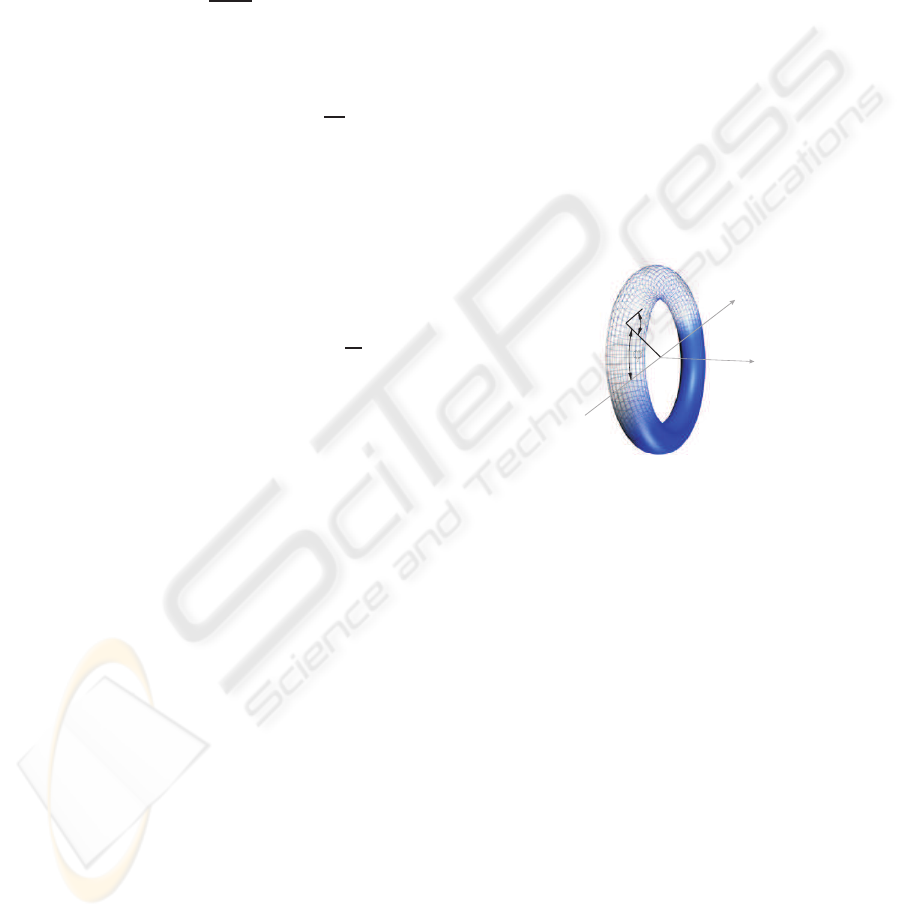
Figure 3: Experimental cell for shoe bottom roughing.
The prototype of the cell is shown in figure
3. It consists of the Mitsubishi Pa10 robot with a
force/torque sensor Jr3 mounted in the robot wrist, a
grinding machine, a Pa10 robot controller and a cell
control computer, which coordinates the task and cal-
culates the required robot torques. The control com-
puter is connected to the robot controller using Arc-
Net. The frequency rate of the control algorithm (Eq.
9) and the motion optimization algorithm (Eq. 15)
is 700 Hz. The grinding path is obtained from CAD
model of the shoe. For this purpose, the control com-
puter is connected to the shoe database computer us-
ing Ethernet. Unfortunately, CAD model itself can
not supply all necessary data for the grinding process.
CAD models are usually available for the reference
shoe size, therefore, non-linear grading of the shoe
shape is necessary for the given size. Additionally,
some technological parameters such as material char-
acteristics and shoe sole gluing technology have to
be taken into account during the grinding trajectory
preparation. For this purpose, we have developed a
special CAD expert program, which enables the op-
erator to define additional technological and material
parameters. The program then automatically gener-
ates the grinding trajectory.
In order to show the efficiency of the proposed al-
gorithm, we defined the shoe grinding trajectory as
seen in the Fig 4. Note that without using trajectory
optimization is is very hard to execute the given task
without splitting the desired trajectory in two or more
fragments. Fig 5 shows how the system rotated joints
of virtual mechanism in order to avoid the joint lim-
its and to minimize joint velocities of the robot and
virtual mechanism.
Similar behavior could be obtained also by using
the well known hybrid force-position control, where
restricted coordinates are perpendicular to the grind-
ing disc. However, the approach with hybrid force-
position control has several disadvantages. First of
−50
0
50
100
150
200
−20
0
20
40
90
100
110
x
y
z
Figure 4: Shoe grinding trajectory.
0 2 4 6 8 10 12 14 16
−10
−5
0
5
10
15
VIRTUAL JOINTS q(8) and q(9)
time(s)
angle(deg)
q8
q9
Figure 5: Virtual mechanism angles q8 and q9.
Figure 6: Resulting forces during the shoe grinding.
all, it requires perfect force tracking in order to main-
tain the tool always perpendicularto the grindingdisc.
Due to the irregularities of the shoe bottom and the
griding disc rotation, this is very hard to obtain. Re-
sults of the force tracking shown in Fig. 6 clearly
demonstrates, that the resulting force tracking is still
imperfect despite of the high sampling frequency of
the control algorithm. Note that only the force in z
direction was controlled in this case. On the contrary,
our approach does not require force control to follow
the shape of the grinding disc at all. Therefore, we
were able to apply the impedance control law, which
is more appropriate for the applications such as grind-
ing and polishing.
6 CONCLUSIONS
In the paper we presented a cell for shoe grinding op-
eration. We proposed a new method of solving the
kinematic redundancy which arises from the shape
SHOE GRINDING CELL USING VIRTUAL MECHANISM APPROACH
163

of the work tool. The main benefit of the proposed
method is the simplicity and efficiency. It can be
used on the existing robot controllers with very mod-
erate changes of the control algorithm. The proposed
method can be applied even in the case of moving ob-
stacles during the task execution, assuming that the
shape and position of the obstacle is known. Another,
perhaps for the practical implementation even more
attractive possibility is to use the proposed approach
in the trajectory generation and not in the control al-
gorithm. In this case we can use existing standard in-
dustrial robots and we benefit from the the advantages
of the kinematic redundancy due to circular shape of
the tool. This latter approach was successfully im-
plemented in the cell for custom finishing operations
in shoe assembly (Nemec and Zlajpah, 2008). It was
also demonstrated that the proposed control has many
advantages when compared with the hybrid force-
position control, which tracks an unknown shape us-
ing only the force sensor data.
REFERENCES
Asada, H. and Slotine, J.-J. (1986). Robot Analysis and
Control. John Wiley & Sons.
Chaumette, F. and Marchand, . (2001). A redundancy-based
iterative approach for avoiding joint limits: Appli-
cation to visual servoing. In IEEE Transactions on
Robotics and Automation, 17(5).
Dulio, S. and Boer, S. (2004). Integrated production plant
(ipp): an innovative laboratory for research projects in
the footwear field. In Int. Journal of Computer Inte-
grated Manufacturing, 17(7) : 601-611.
Jatta, F., Zanoni, L., Fassi, I., and Negri, S. (2004). A rough-
ing/cementing robotic cell for custom made shoe man-
ufacture. In Int. J. Computer Intergrated Manufactur-
ing, 17(7) : 645–652.
Khatib, O. (1986). Real-time obstacle avoidance for ma-
nipulators and mobile robots. In Int. J. of Robotic Re-
search, 5 : 90 – 98.
Khatib, O. (1987). A unified approach for motion and force
control of robot manipulators:the operational space
formulation. In IEEE Trans. on Robotics and Automa-
tion, 3(1) : 43 – 53.
Nemec, B. and et all (2003). Technology fostering indi-
vidual, organisational, and regional development: an
international perspective.
Nemec, B. and Zlajpah, L. (2000). Null velocity control
with dinamically consistent pseudo-inverse. In Robot-
ica, 18 : 513 – 518.
Nemec, B. and Zlajpah, L. (2001). Experiments with force
control of redundant robots in unstructured environ-
ment using minimal null-space formulation. In Jour-
nal of Advanced Computational Intelligence, 5(5) :
263 – 268.
Nemec, B. and Zlajpah, L. (2008). Robotic cell for custom
finishing operations. In Int. J. Computer Intergrated
Manufacturing, 21(1) : 33–42.
Nemec, B., Zlajpah, L., and Omrcen, D. (2007). Compar-
ison of null-space and minimal null-space control al-
gorithms. In Robotica, 2007, 25(5):511–520.
Nenchev, D. N. (1989). Redundancy resolution through lo-
cal optimization: A review. In J. of Robotic Systems,
6(6) : 769 – 798.
Oh, Y., Chung, W., Youm, Y., and Suh, I. (1998). Exper-
iments on extended impedance control of redundant
manipulator. In Proc. IEEE/RJS Int. Conf. on Intelli-
gent Robots and Systems, : 1320 – 1325, Victoria.
Park, J., Chung, W., and Youm, Y. (2002). Characterization
of instability of dynamic control for kinematically re-
dundant manipulators. In Proc. IEEE Conf. Robotics
and Automation, : 2400 – 2405, Washington DC.
Taylor, P. and Taylor, G. (1988). Garments and Shoe Indus-
try Robots.
ICINCO 2008 - International Conference on Informatics in Control, Automation and Robotics
164
