OBTAINING MINIMUM VARIABILITY OWA OPERATORS

UNDER A FUZZY LEVEL OF ORNESS

Kaj-Mikael Björk

Department of Technology, IAMSR, Åbo Akademi University

Joukahaisenkatu 4-6A, 20520 Turku, Finland

Keywords: OWA operators, Fuzzy numbers, Optimization, Signed distance-defuzzification.

Abstract: Finding the optimal OWA (ordered weighted averaging) operators is important in many decision support

problems. The OWA-operators enables the decision maker to model very different kinds of aggregator

operators. The weights need to be, however, determined under some criteria, and can be found through the

solution of some optimization problems. The important parameter called the level of orness may, in many

cases, be uncertain to some degree. Decision makers are often able to estimate the level using fuzzy

numbers. Therefore, this paper contributes to the current state of the art in OWA operators with a model that

can determine the optimal (minimum variability) OWA operators under a (unsymmetrical triangular) fuzzy

level of orness.

1 INTRODUCTION

Information aggregation is used in many

applications. Some fields of research that takes

advantage of aggregation may be found in Neural

Networks, fuzzy logic controllers, multi-criteria

optimisation and more. Aggregation is necessary to

logically split up entities onto several units. A very

eminent way of doing aggregators is the OWA

operators, originally described by (Yager, 1988). He

defined a weight, w

, to be associated with an

ordered position of the aggregate. The weights are

often ordered such that the best criterion is

associated with the first weight and so on. Given the

weights for each object, Yager defined a level of

orness, which will represent a major characteristic of

the weighting structure. An orness-value of zero

represents a situation that the weakest criterion has

the full weight, whereas an orness-value of one

represents the opposite, i.e. the strongest criterion

has the full weight.

Finding the optimal distribution of the weights

under a certain level of orness has obtained some

interest during the last decade. The weights can be

optimal in many ways; O’Hagan, for instance

(1988), presented a numerical method to find the

maximum entropy OWA operators under a crisp

level of orness. Quite recently (Fuller and

Majlender, 2001), (Fuller and Majlender, 2003) and

(Carlsson et al., 2003) extended those results with

both a analytical model for the maximum entropy

problem as well as an analytical solution to the

minimum variability problem. These contributions

are interesting and sound theoretical findings. They

did not, however, consider a fuzzy level of orness.

The level of orness is often estimated from expert

opinions and can be inherent fuzzy. Therefore, this

paper contributes with a fuzzy orness level,

minimum variability, OWA operator model. This

paper does not use the Lagrange multiplier method,

used by (Fuller and Majlender, 2001, 2003), but

instead the constraints for the minimum variability

problem are substituted in the objective function.

Afterwards, the objective function is assumed to

have a triangular fuzzy level of orness. This paper

uses the signed distance method (Yao and Wu,

2000) to defuzzify the objective function, where

after the optimisation problem is checked for

convexity and solved numerically to the optimal

solution. Other contributions using the signed

distance method to defuzzify fuzzy numbers are

(Salameh and Jaber, 2000) and (Yao and Chiang,

2003), for instance.

The paper is organised as follows: first the

minimum variability OWA operator problem is

formulated. Then the problem is altered to contain

only an objective function, where after the level of

orness is allowed to be fuzzy, but defuzzified in

114

Björk K. (2008).

OBTAINING MINIMUM VARIABILITY OWA OPERATORS UNDER A FUZZY LEVEL OF ORNESS.

In Proceedings of the Fifth International Conference on Informatics in Control, Automation and Robotics - ICSO, pages 114-119

DOI: 10.5220/0001483501140119

 SciTePress

order to obtain a crisp optimal solution to the

problem. Finally, a small problem is solved and

compared with the solution obtained by (Fuller and

Majlender, 2003).

2 THE MINIMUM VARIABILITY

OWA OPERATOR PROBLEM

According to (Fuller and Majlender, 2003), the

minimum variability problem is the following:

10,

)(..

min

≤≤=

−

∑

wornessts

αα

(1)

where w

is the positive weigths (the variables in the

optimisation problem) and n is the total number of

weights. α is the level of orness (parameter in the

optimisation problem). This model can be solved

analytically to optimum using a Lagrange multiplier

method as in Fuller and Majlender (2003).

The model in eq. (1) can be reformulated by

substituting each of the two constraints into the

objective function. The second constraint in (1) will

give us the following relationship:

∑

−=

(2)

Subsituting (2) into (1) yields

111

min

⎟

⎠

⎞

⎜

⎝

⎛

−+

−

⎟

⎠

⎞

⎜

⎝

⎛

−+−

∑∑

(3)

The constraint in (3) will give us the following

relationship:

() ( )( )

−−+−−=

∑

111

nwiw

(4)

Using (4) in (3) will give us the simplified

optimisation problem, containing only an objective

function as follows (after some simplifications)

()

min

⎟

⎠

⎞

⎜

⎝

⎛

−+++−−+

⎟

⎠

⎞

⎜

⎝

⎛

−−−−++

−

∑

winn

αα

(5)

First of all it is worth noticing that the optimisation

problem in eq. (5) is convex. The convexity can be

established by examining the terms and since

classical convexity theory states that a function

∑

kxcxf

)()( , is always convex, where c

and

k are constants.

The next step is to manipulate (5) to remove the

squares (in order to be able to defuzzify it with the

signed distance method). This will result (after some

simplifications and rearrangements) in the following

problem (i.e. to an equivalent problem to the one

found in eq. 5):

There are some intermediate steps between eqs. (5)

and (6) that are left out since it would require some

additional pages of formulas. The reformulation of

eq. (5) into the problem in eq. (6) may seem to

complicate the problem structure, but in fact it helps

the defuzzification step, since α will only be found

in separate terms.

()

() ()

()

wwji

wiwii

∑∑

∑

∑∑

−

=+=

−

=+=

−−+

−+

−+−−

−−+−+

−−−−+

++++−

)2(2

)1(1

64662

664410

222

min

ααα

(6)

OBTAINING MINIMUM VARIABILITY OWA OPERATORS UNDER A FUZZY LEVEL OF ORNESS

115

3 DEFUZZIFICATION OF THE

ORNESS VALUE

If the α value (the orness value) is triangular fuzzy,

denoted as

, the optimization problem becomes

simply the following:

Some basics from fuzzy set theory need to be

introduced in order to make the following model

development self-contained.

Definition 1.

Consider the fuzzy set

),,(

cbaA = where cba

< and defined on R,

which is called a triangular fuzzy number, if the

membership function of

is given by

⎪

⎩

⎪

⎨

⎧

≤≤−−

.,0

),/()(

,),/()(

)(

otherwise

cxbbcxc

bxaabax

Definition 2. Let B

be a fuzzy set on R and

10 ≤≤

. The α

-cut of B

is all the points x such

that

≥)(

, i.e.

{}

xxB

αμα

≥= )()(

In order to find non-fuzzy values for the model

we need to use some distance measures and we will

use the signed distance (Yao and Wu, 2000).

Definition 3. For any a and R∈0 , the signed

distance from

a to 0 is aad =)0,(

. And if 0

a ,

the distance from

a to 0 is )0,(

ada −=

−

Let

be the family of all fuzzy sets B

defined

on R for which the α-cut

[]

)(),()(

cUcLc

BBB

exists for every

[

]

1,0

∈

, and both )(

and

)(

are continuous functions on

[

]

1,0

∈

Then, for any

∈

, we have (see Chang, 2004, for

instance)

[

]

)(,)(

≤≤

cUcL

BBB

αα

From Chang (2004) it can be finally stated

(originally by results from Yao and Wu, 2000) how

to calculate the signed distances.

Definition 4. For

∈

define the signed

distance of

[]

∫

.)()(

(

ccUcL

dBBBd

ααα

The Definition 3 will give us several properties

of which the most important is

Property 1. Consider the triangular fuzzy

number

),,(

cbaA = : the α-cut of

[

]

)(),()(

cUcLc

AAA

ααα

= , for

[]

1,0∈

, where

ccL

abaA

)()(

−

and

ccU

bccA

)()(

−

−= ,

the signed distance of

).2(

(

cbaAd ++=

Let us assume that we have a triangular fuzzy

orness level, i.e.

),,(

Δ+

−

(8)

(Note that the orness value, α , should not be mixed

up with the α-cut, called α

.) Then we will

defuzzify

in two different ways, depending on

whether

is squared or not. From Property 1 we

will get directly that the signed distance of

[]

Δ−Δ+=

Δ+++Δ−=

)(2)(

(

αααα

(9)

And according to Definition 4 we will get that the

signed distance for

will be

()

() ()

()

wwji

wiwii

∑∑

∑

∑∑

−

=+=

−

=+=

−−+

−+

−+−−

−−+−+

−−−−+

++++−

)2(2

)1(1

64662

min

ααα

(7)

ICINCO 2008 - International Conference on Informatics in Control, Automation and Robotics

116

() ()

[]

()

chchchh

hchh

clclclcl

llcll

chh

cll

ccUcL

αααα

ααααα

αα

αααααα

∫

⎥

⎦

⎤

⎢

⎣

⎡

Δ+

Δ+Δ−Δ−Δ+

Δ+Δ−Δ++

Δ+Δ−Δ+Δ−

⎥

⎦

⎤

⎢

⎣

⎡

Δ−Δ++

Δ+Δ−

222

)()(

(

(10)

Finally we will get the signed distance value for

(

hlhl

d Δ+Δ+Δ+Δ−=

αααα

(11)

The defuzzified objective function will be

And putting the signed distances (to defuzzify) of

and

respectively (Equations 9 and 11), into

eq. (7) will give us the final defuzzified objective

function as

()

() ()

()

lhi

hlhl

wwji

wiwi

wii

∑∑

∑

−

=+=

−

=+=

−−+

−

⎟

⎠

⎞

⎜

⎝

⎛

Δ−Δ++−+

−

Δ−Δ+

−−−

+−+−

Δ−Δ+

−

⎟

⎠

⎞

⎜

⎝

⎛

Δ−Δ+⋅−

⎟

⎠

⎞

⎜

⎝

⎛

Δ+Δ+Δ+Δ−−

⎟

⎠

⎞

⎜

⎝

⎛

Δ−Δ+++

⎟

⎠

⎞

⎜

⎝

⎛

Δ+Δ+Δ+Δ−⋅+

Δ+Δ+Δ+Δ−

+−

)2(2

)1(1

662

min

ααα

(13)

The fuzzy minimum variability OWA operator

problem can thus be solved by minimizing eq. (13).

The first and second weight can there-after be

obtained from eqs. (4) and (2), respectively (with the

defuzzified value of

, and not the crisp one, c.f.

eq. 14).

() ( )

()

(111

dnwiw

−−+−−=

∑

(14)

It is worth noticing that the convexity will remain

(from eq. 5) through the operations, since the effect

of a fuzzy orness-value (α-value) will only affect the

constant in the optimization problem. (I.e. it will

only affect the parameter

k in the functions of the

form

∑

kxcxf

)()( and, thus, not affect the

convexity. In addition, the operations in eqs. 6-13

will not change the convexity assumption.) The

optimization problem in eq. (13) can be solved

numerically with any local nonlinear optimization

methods, which can guarantee local optimal

convergence. The method need not be able to handle

constraints, since there are no constraints involved in

eq. (13), except for the non-negativity constraint of

the variables. A method that can handle simple

()

() ()

()

wwji

widwi

wii

dndd

∑∑

∑

−

=+=

−

=+=

−−+

−+−+

−−−−

+−+−−

⋅−−++

⋅+++−

)2(2

)1(1

64)0

(53

(

662

(

(4)0

(10

(

min

ααα

(12)

OBTAINING MINIMUM VARIABILITY OWA OPERATORS UNDER A FUZZY LEVEL OF ORNESS

117

constraints is, however, advisable so that the

substituted constraints in eqs. (2) and (4) will always

get non-negative values.

4 EXAMPLE

In this section, a test problem is solved and

compared to the crisp solution by Fuller and

Majlender (2003). This problem contains 5 weights

and it is calculated for a level of orness (α-value) of

0.1, 0.2, 0.3, 0.4 and 0.5. First, the problem is

compared to the crisp solution for an α-value of 0.3

and different values of the Δ-parameters (i.e.

different fuzziness values). The solution is obtained

by using a standard local search method on the

problem in eq. (13). The problem in this paper is

solved with the extended Newton method found in

the standard solver available in Microsoft Excel.

Table 1: The optimal OWA-operators for different

fuzziness values (α=0.3).

Obj

0.300 0.000 0.000 0.040 0.120 0.200 0.280 0.360 0.013

0.300 0.050 0.050 0.040 0.120 0.200 0.280 0.360 0.018

0.300 0.100 0.050 0.030 0.115 0.200 0.285 0.370 0.027

0.300 0.050 0.100 0.050 0.125 0.200 0.275 0.350 0.024

In Table 1 it should be noted that the crisp case (i.e.

when the Δ’s are 0) collapses to the same solution as

reported in Fuller and Majlender (2003). It should

also be noted that the optimal solution (in this

example) remained the same as the crisp solution if

= Δ

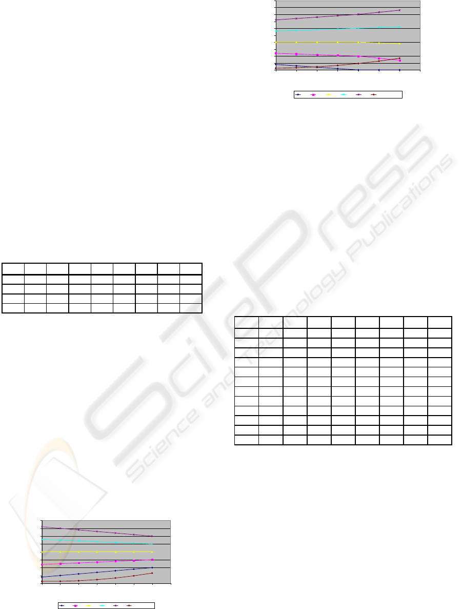
. In order to illustrate the behaviour of the

weights for different Δ-values (as well as the

objective function), Figure 1 and Figure 2 are

included. In these figures, the α-value is set to 0.3,

but one of the Δ-values is allowed to change. One

can see in Figure 1 that if Δ

is increased from 0 to

0.3 the objective value increases from 0.013 to 0.065

and the weights get more similar to each other. In a

similar manner when Δ

increasing from 0 to 0.3, the

objective value will increase from 0.013 to 0.084

and the weights become more diverse.

0.000

0.050

0.100

0.150

0.200

0.250

0.300

0.350

0.400

0.000 0.050 0.100 0.150 0.200 0.250 0.300 0.350

Δh

w1 w2 w3 w4 w5 Obj. value

Figure 1: The sensitivity analysis of Δ

for α=0 and Δ

=0.

0.000

0.050

0.100

0.150

0.200

0.250

0.300

0.350

0.400

0.450

0.500

0.000 0.050 0.100 0.150 0.200 0.250 0.300 0.350

Δl

w1 w2 w3 w4 w5 Obj. value

Figure 2: The sensitivity analysis of Δ

for α=0 and Δ

=0.

In Table 2, the optimal OWA-operators for several

α-values are calculated. When the Δ

= Δ

= 0, (i.e. the

crisp case) the operator-values are the same as the

one reported by Fuller and Majlender (2003). In the

case of Δ-values greater than zero (and unequal) the

operator-values are different from the crisp case,

except for the case of α=0.1. It is also worth noticing

that the objective value for the crisp case is always

better than for the fuzzy cases (in this example);

when α=0.1 the increase is only about 20 %, but

with bigger α-values, the bigger the increase in the

objective function when fuzziness is introduced.

Table 2: The optimal OWA-operators for different α-

values as well as fuzziness values.

Obj

0.100 0.000 0.000 0.000 0.000 0.033 0.333 0.633 0.063

0.100 0.050 0.100 0.000 0.000 0.058 0.333 0.608 0.069

0.100 0.100 0.050 0.000 0.000 0.008 0.333 0.658 0.081

0.200 0.000 0.000 0.000 0.040 0.180 0.320 0.460 0.030

0.200 0.050 0.100 0.000 0.055 0.185 0.315 0.445 0.039

0.200 0.100 0.050 0.000 0.025 0.175 0.325 0.475 0.045

0.400 0.000 0.000 0.120 0.160 0.200 0.240 0.280 0.003

0.400 0.050 0.100 0.130 0.165 0.200 0.235 0.270 0.015

0.400 0.100 0.050 0.110 0.155 0.200 0.245 0.290 0.016

0.500 0.000 0.000 0.200 0.200 0.200 0.200 0.200 0.000

0.500 0.050 0.100 0.210 0.205 0.200 0.195 0.190 0.012

0.500 0.100 0.050 0.190 0.195 0.200 0.205 0.210 0.012

5 CONCLUSIONS

This paper presents a new fuzzy minimum

variability model for the OWA-operators, originally

introduced by Yager (1988). Previous results in this

line of research is the elegant results by Fuller and

Majlender (2001, 2003), where both the minimum

variability problem as well as the maximum entropy

problem were solved. These results assumed,

however, a crisp level of orness.

This paper added the current research track a

model that could account for unsymmetrical (or

symmetrical) triangular fuzzy levels of orness. This

is important if the decision maker is not certain

ICINCO 2008 - International Conference on Informatics in Control, Automation and Robotics

118

about the level of orness, but can estimate it through

the proposed fuzzy numbers. The minimum

variability model for the fuzzy orness level is

obtained through a slightly different approach than

the one used in Fuller and Majlender (2001, 2003).

This paper substitutes the constraints in the problem

(c.f. eq. 1) such that the variables w

and w

are

eliminated out of the problem, and after some

rearrangements a convex objective in smaller

dimension remains of the original problem. This

problem is allowed to have triangular fuzzy α-

values, but in order to solve the optimisation

problem, the α-values are defuzzified with the

signed distance method. The defuzzified

optimization problem is then solved with a

numerical optimisation method that can guarantee

local convergence. The first two weights are then

solved from the substituted constraints.

The future research consists of analytical

solutions for the optimization problem as well as

extending the level of orness to contain other types

of fuzzy numbers than the triangular ones. A natural

extension could be to investigate the trapezoidal

fuzzy numbers as well as other defuzzification

methods.

REFERENCES

Carlsson C, Fuller R. & Majlender P., 2003. A note on

constrained OWA aggregation. Fuzzy sets and

systems, 139, pp. 543-546.

Chang H-C., 2004. An application of fuzzy sets theory to

the EOQ model with imperfect quality items.

Computers & Operations Research, 31, pp. 2079-

2092.

Fuller R. & Majlender P., 2001. An analytical approach

for obtaining OWA-operator weights. Fuzzy sets and

systems, 124, pp. 53-57.

Fuller R. & Majlender P., 2003. On obtaining minimum

variability OWA operator weights. Fuzzy sets and

systems, 136, pp. 203-215.

O’Hagan M., 1988. Aggregating template or rule

antecedents in real-time expert systems with fuzzy set

logic. Proceedings of 22

annual Asilomal conference

on signals, systems and computers, pp. 681-689.

Salameh M.K. and Jaber M.Y., 2000. Economic

production quantity model for items with imperfect

quality. Int. Journal of Production Economics, 64,

pp.59-64.

Yager R.R., 1988. Ordered weighted averaging

aggregation operators in multi-criteria decision

making. IEEE Transactions on Systems, Man, and

Cybernetics, 18, pp. 183-190.

Yao J.S. and Wu K., 2000. Ranking fuzzy numbers based

on decomposition principle and signed distance, Fuzzy

Sets and Systems, 116, pp. 275-288.

Yao J-S and Chiang J., 2003. Inventory without backorder

with fuzzy total cost and fuzzy storing cost defuzzified

by centroid and signed distance. European Journal of

Operational Research, 148, pp. 401-409.

OBTAINING MINIMUM VARIABILITY OWA OPERATORS UNDER A FUZZY LEVEL OF ORNESS

119