LIGHT-WEIGHT REINFORCEMENT LEARNING WITH

FUNCTION APPROXIMATION FOR REAL-LIFE CONTROL TASKS

Kary Främling

Helsinki University of Technology, PL 5500, FI-02015, Finland

Keywords:

Reinforcement learning, function approximation, normalised radial basis function network, eligibility trace,

mountain-car, cart-pole, pendulum.

Abstract:

Despite the impressive achievements of reinforcement learning (RL) in playing Backgammon already in the

beginning of the 90’s, relatively few successful real-world applications of RL have been reported since then.

This could be due to the tendency of RL research to focus on discrete Markov Decision Processes that make

it difﬁcult to handle tasks with continuous-valued features. Another reason could be a tendency to develop

continuously more complex mathematical RL models that are difﬁcult to implement and operate. Both of these

issues are addressed in this paper by using the gradient-descent Sarsa(λ) method together with a Normalised

Radial Basis Function neural net. The experimental results on three typical benchmark control tasks show that

these methods outperform most previously reported results on these tasks, while remaining computationally

feasible to implement even as embedded software. Therefore the presented results can serve as a reference

both regarding learning performance and computational applicability of RL for real-life applications.

1 INTRODUCTION

A Reinforcement Learning (RL) agent can sense the

state of itself and its environment, take actions that

may change that state in some way and improve its

behaviour based on a reward signal that expresses if

one or several actions (or their result) was good or

bad and to what extent. RL is therefore similar to the

way that most animals learn to handle new or chang-

ing situations, e.g. babies learning how to walk and

grab things, children learning how to ride a bicycle

or adults learning how to drive a car. Despite this

relationship with human and animal learning in the

real world, it is surprising how few successful uses of

RL for real-world control applications have been re-

ported. The most well-known success of RL so far

might be the TD-Gammon system (Tesauro, 1995)

that learned to play Backgammon on world-champion

level. However, Backgammon is not a control task

and the methods and results are not easy to extrapolate

to control tasks. A recent success on a real-world RL

control task is the helicopter ﬂight control reported in

(Abbeel et al., 2007). What is common to both of

these successful applications of RL (especially in he-

licopter ﬂight) is that they are the result of rather com-

plex calculations that involve several different learn-

ing phases and extensive hand-tuning by human de-

signers. Even in experiments with standard control

tasks such as those used in this paper, the RL meth-

ods employed tend to be complex and require exten-

sive hand-tuning by human designers in order to make

the learning task feasible. This complexity makes it

difﬁcult to re-use successful RL models in new appli-

cation areas. Such models also tend to be too complex

to provide plausible models of animal learning.

Both TD-Gammon and the helicopter controller

use function approximation in order to be able to

handle the huge state spaces involved. Especially

continuous-valued control tasks tend to be problem-

atic for RL because of their inﬁnite state space. Many

popular RL methods assume that the task to learn can

be represented as a Markov Decision Process (MDP).

In tasks with continuous-valued inputs it becomes

necessary to discretize the state space in order to han-

dle it as an MDP but the discretisation easily leads

to an explosion of the state space. This contradic-

127

Främling K. (2008).

LIGHT-WEIGHT REINFORCEMENT LEARNING WITH FUNCTION APPROXIMATION FOR REAL-LIFE CONTROL TASKS.

In Proceedings of the Fifth International Conference on Informatics in Control, Automation and Robotics - ICSO, pages 127-134

DOI: 10.5220/0001484001270134

 SciTePress

tion between ‘provably converging’ but ‘hard-to-use

in real-life’ MDP-based methods may also be a rea-

son for the lack of reported successful uses of RL in

real-world control tasks.

In this paper we will show how function ap-

proximation and one of the ‘lightest’ RL methods,

i.e. model-free action-value learning with gradient-

descent Sarsa(λ), can be used for successful learning

of three benchmark control tasks. Less hand-tuning is

needed and learning is signiﬁcantly faster than in pre-

viously reported experiments. These small memory

and computation requirements and the rapid learning

should make it possible to use RL even in embed-

ded systems that could adapt to their environment.

These characteristics also make the learning biologi-

cally plausible. The experimental tasks used are the

Mountain-Car, Swinging up pendulum with limited

torque and Cart-Pole tasks.

After this introduction, section 2 describes the

background and theory of gradient-descent Sarsa(λ),

then section 3 presents the Normalized Radial Basis

Function approximation technique used, followed by

experimental results in section 4 and conclusions.

2 ACTION-VALUE LEARNING

WITH FUNCTION

APPROXIMATION

Action-value learning is needed in control tasks

where no model of the controlled system is available.

In the case of continuous-valued function approxi-

mation, gradient-descent Sarsa(λ) (Sutton and Barto,

1998, p. 211) can be used:

t+1

+ α[r

t+1

+ γQ

t+1

) − Q

)]~e

(1)

where

is the parameter vector of the function ap-

proximator, r

t+1

is the reward received upon entering

a new state, α is a learning rate, γ is the discount rate

and Q

) and Q

t+1

) are the action-value

estimates for the current and next state, respectively.

In the case of an accumulating trace, the trace ~e

updated according to:

= γλ~e

t−1

+ ∇

) (2)

with~e

0. ∇





, for any function f denotes the

vector of partial derivatives (Sutton and Barto, 1998,

p. 197):





∂f





∂θ

(1)

∂f





∂θ

(2)

,...,

∂f





∂θ

(n)





, (3)

where

φ is feature vector that consist of the state vari-

ables of the task (continuous-valued or not). Eligi-

bility traces can speed up learning signiﬁcantly by

improving temporal credit assignment. They are in-

spired from the behaviour of biological neurons that

reach maximum eligibility for learning a short time

after their activation and were mentioned in the con-

text of Machine Learning at least as early as 1972 and

used for action-value learning at least as early as 1983

(Barto et al., 1983), where the accumulating eligibil-

ity trace for discrete state tasks (MDP) was proposed:

(s,a) =



γλe

t−1

(s,a) + 1

s = s

and

a = a

;

γλe

t−1

(s,a)

otherwise

(4)

for all s,a. λ is a trace decay parameter. s corresponds

to the feature vector

φ in 3 but is restricted to binary

values. Equation 4 is a special case of equation 2

when using binary state representations because then

∇

) = 1 when s = s

and a = a

and zero oth-

erwise. In (Singh and Sutton, 1996) it was proposed

to use a replacing eligibility trace instead of the accu-

mulating eligibility trace:

(s,a) =







s = s

and

a = a

;

s = s

and

a 6= a

;

γλe

t−1

(s,a)

s 6= s

(5)

The replacing eligibility trace outperformed the accu-

mulating eligibility trace in the Mountain-Car task as

reported in (Singh and Sutton, 1996). This is the main

reason why replacing traces are considered to perform

better than accumulating traces. In (Främling, 2007b)

a generalisation was proposed for the replacing trace

that makes it possible to use with continuous-valued

function approximation:

= max(γλ~e

t−1

,∇

)) (6)

As for the accumulating trace, equation 5 is identical

to equation 6 in the case of binary features, except

for resetting the trace of unused actions of the current

state to zero in equation 5. Even though the results

in (Främling, 2007b) seem to conﬁrm the advantage

of replacing traces, especially when not resetting the

traces of unused actions, there is still a lack of evi-

dence on whether this is also true for other tasks. The

experiments in this paper are performed using both

kinds of eligibility traces as an attempt to provide in-

creased insight into this issue.

ICINCO 2008 - International Conference on Informatics in Control, Automation and Robotics

128

3 NORMALISED RADIAL BASIS

FUNCTION NETWORK

APPLIED TO ACTION-VALUE

LEARNING

When function approximationwith neural nets is used

for learning an action-value function, an eligibility

trace value is associated with every weight of the neu-

ral net (Barto et al., 1983). Then the eligibility trace

value reﬂects to what extent and how long ago the

neurons connected by the weight have been activated.

The use of function approximation rather than binary

lookup-tables signiﬁes that more than one feature

value φ can be different from zero. This is also the

case with the binary CMAC (Cerebellar Model Artic-

ulation Controller) neural network (Albus, 1975) used

in (Singh and Sutton, 1996). When using CMAC,

there are as many active features as there are over-

lapping layers in the CMAC, which could lead to

excessive weight changes in Equation 1. In order

to avoid this, (Singh and Sutton, 1996) divide every

value e

(s,a) by the sum of all feature values in or-

der to avoid learning divergence as a result of exces-

sive weight changes. No justiﬁcation was given for

this operation in (Singh and Sutton, 1996) but there

seems to be a connection with the well-known Nor-

malised Least Mean Squares (NLMS) method, where

α in Equation 1 is replaced by α

norm

= α/

∑

. (7)

The use of NLMS for RL in a real-world robotics task

has been studied e.g. in (Främling, 2004) and (Främ-

ling, 2005). When using continuous-valued function

approximation, most terms ∇

) in equation

2 will be different both from zero and one, which is

the main source of incompatibility between the dis-

crete eligibility traces (Equations 4 and 5) and their

continuous-valued counterparts (Equations 2 and 6).

In order to avoid weight divergence in equation 1,

it can be assumed that an NLMS-type normalisation

would be useful also with continuous-valuedfeatures.

Because NLMS does not seem to have been used in

neural nets, another kind of normalisation than NLMS

is used here, i.e. the Normalised Radial Basis Func-

tion network (NRBF).

The continuous feature values are calculated by an

RBF network as:

(~s

) = exp



−

(~s

−~c)



, (8)

where~c is the centroid vector of the RBF neuron and

is the spread parameter. The action-value estimate

of action a is:

(~s

,a) =

∑

i=1

∑

k=1

, (9)

where w

is the weight between the ‘action’ neuron a

and the RBF neuron i. The division by

∑

k=1

, where

N is the number of RBF neurons, is the normalisation

step that ensures that the sum of all φ will be exactly

one. Every parameter w

, has its corresponding eli-

gibility trace value. For the accumulating trace, equa-

tion 2 was used in all experiments, while equation 6

was used for the replacing trace. In all experiments,

an afﬁne transformation mapped the actual state val-

ues from the respective value ranges into the range

[0,1] that was used as ~s. This transformation makes

it easier to adjust the spread parameter (r

= 0.01 is

used in all experiments).

4 EXPERIMENTS

The Mountain-Car task (Figure 1) was used in (Singh

and Sutton, 1996) and the results presented there

seem to be the main reason why replacing eligibil-

ity traces are considered to perform better than accu-

mulating traces. The second task consists in swing-

ing up a pendulum with limited torque and keep-

ing it in upright position (Figure 4). The pendu-

lum task is surprisingly difﬁcult for ordinary learn-

ing methods such as Sarsa(λ) with binary represen-

tations (lookup-table, CMAC) due to the non-linear

control function required for passing from swing-

up behaviour to balance-keeping behaviour. For the

Cart-Pole task (Figure 7), successful results were re-

ported using actor-critic and lookup-tables already in

(Barto et al., 1983).

For each task, results are ﬁrst shown by graphs

that allow comparison between results shown here

and those reported in existing literature. A supple-

mentary graph may be used to show the results in

a homogeneous way between the three tasks that al-

lows to evaluate both learning speed and ﬁnal perfor-

mance after learning, as well as how well the accumu-

lating and the replacing traces perform in each task.

These graphs are also intended to provide a uniform

benchmark framework for future experiments using

the same tasks.

4.1 Mountain-Car

One of the ﬁrst presentations of this task seems to be

in (Moore, 1991), where a model of the environment

was learned. The task description used here is identi-

cal to the one in (Singh and Sutton, 1996). The task

LIGHT-WEIGHT REINFORCEMENT LEARNING WITH FUNCTION APPROXIMATION FOR REAL-LIFE

CONTROL TASKS

129

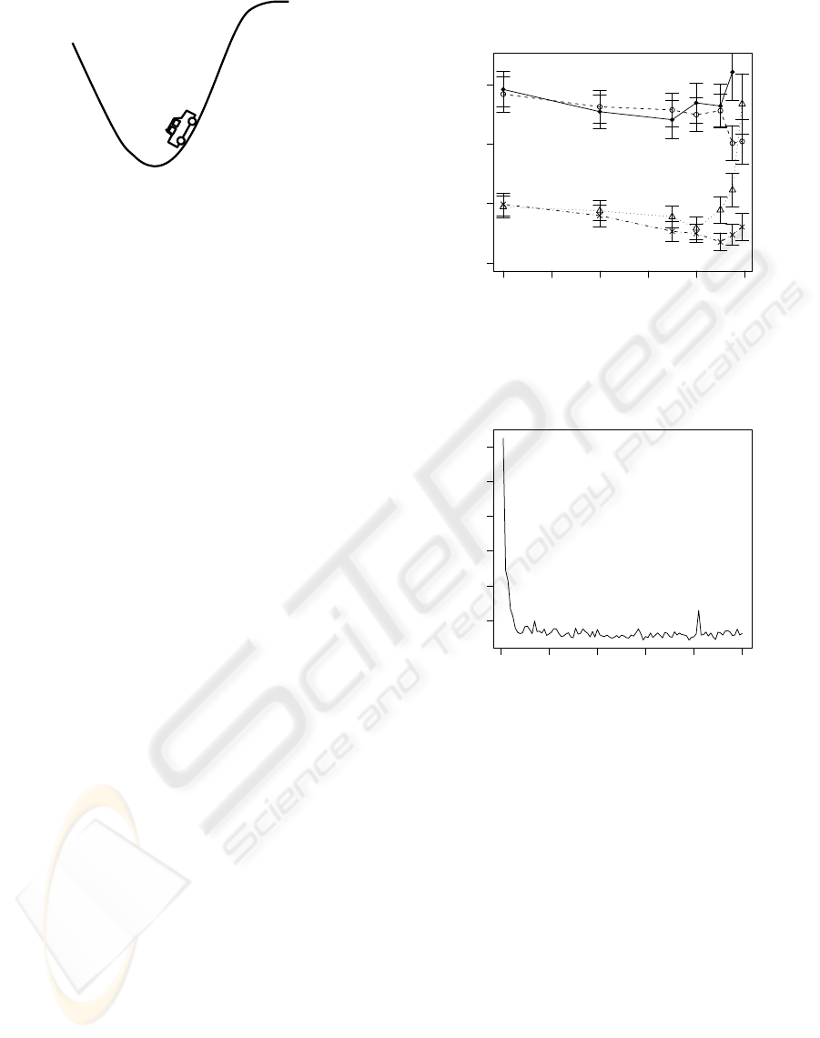
Figure 1: Mountain-Car task.

consists in accelerating an under-powered car up a

hill, which is only possible if the car ﬁrst gains enough

inertia by backing away from the hill. The task has a

continuous-valued state vector ~s

= (x

), i.e. the

position x

and the velocity v

. At the beginning of

each trial these are initialized randomly, uniformly

from the range x ∈ [−1.2,0.5] and v ∈ [−0.07,0.07].

The altitude is sin(3x). 8×8 RBF neurons were used

with regularly spaced centroids. The agent chooses

from three actions {+1, 0, − 1} corresponding to for-

ward thrust, no thrust and reverse. The physics of the

task are:

t+1

bound

+ 0.001a

+ gcos(3x

))

t+1

= max{x

+ v

t+1

,−1.2}

where g = 0.0025 is the force of gravity and the bound

operation places the variable within its allowed range.

If x

t+1

is clipped by the max-operator, then v

t+1

reset to 0. The terminal state is any position with

t+1

> 0.5. The reward function is the cost-to-go

function as in (Singh and Sutton, 1996), i.e. giving -1

reward for every step except when reaching the goal,

where zero reward is given. The weights of the neural

net were set to zero before every new run so the ini-

tial action-value estimates are zero. The discount rate

γ was one.

Figure 2 shows the average number of steps per

episode for the best α values (4.9, 4.3, 4.3, 4.7, 3.9,

3.3 and 2.5) as a function of λ, where the numbers

are averaged for 30 agent runs with 20 episodes each

as in (Singh and Sutton, 1996). For some reason, the

results reported here indicate 50% less steps than in

most other papers (except e.g. (Smart and Kaelbling,

2000) who have similar numbers as here), which

should be taken into consideration when comparing

results. Taking this difference into consideration, the

CMAC results shown in Figure 2 are consistent with

those in (Singh and Sutton, 1996). The results using

gradient-descent Sarsa(λ) and NRBF are signiﬁcantly

better than those obtained with CMAC.

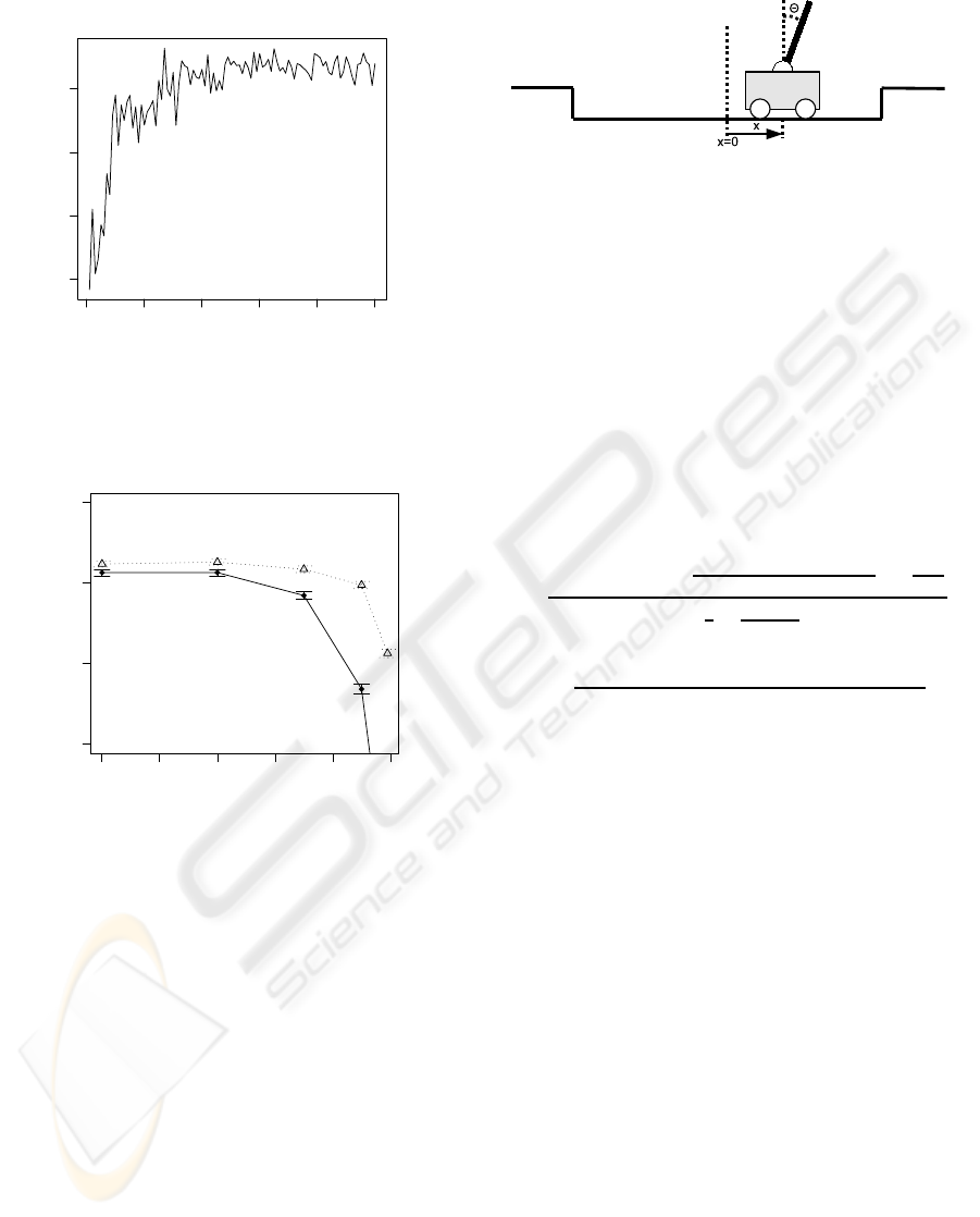
Figure 3 shows the average number of steps per

episode for the best-performing agent with α = 3.9

and λ = 0.9. Convergence to an average of 60 steps

0.0 0.2 0.4 0.6 0.8 1.0

100 150 200 250

Mountain−Car, CMAC and RBF

Average Steps/Episode at best α

CMAC accumulating

CMAC replacing with reset

RBF accumulating

RBF replacing without reset

Figure 2: Average number of steps per episode for 30 agents

running 20 episodes as in (Singh and Sutton, 1996).

0 20 40 60 80 100

100 200 300 400 500 600

Episode

Average Steps/Episode

Figure 3: Average number of steps per episode for best-

performing agent (replacing trace, α = 3.9 and λ = 0.9).

per episode is achieved after about 40 episodes. This

is better than the ‘less than 100 episodes’ indicated in

(Abramson et al., 2003). The optimal number of steps

indicated in (Smart and Kaelbling, 2000) is 56 steps

so 60 steps per episode can be considered optimal due

to the continuing exploration caused by the -1 reward

on every step. Therefore the converged learning re-

sult is also as good as in (Abramson et al., 2003) and

(Schaefer et al., 2007). (Abramson et al., 2003) used

Learning Vector Quantization together with Sarsa in-

stead of using NRBF so the complexity of the learning

algorithm is similar to the one used in this paper. The

reward function provided more guidance towards the

goal than the one used here and a ﬁxed starting point

was used instead of a random one. The neural net

used in (Schaefer et al., 2007) is more complex than

the one used here while a reward of +1 was given at

ICINCO 2008 - International Conference on Informatics in Control, Automation and Robotics

130

Figure 4: Pendulum swing-up with limited torque task.

the goal and zero otherwise. (Smart and Kaelbling,

2000) use an RBF-like neural network together with

Sarsa but no eligibility traces and a reward that is in-

versely proportionalto the velocity at goal (one if zero

velocity) and zero otherwise. Results are indicated

as a function of training steps rather than episodes

but a rough estimate would indicate that convergence

occurs after over 2000 episodes. The experimental

settings and the ways in which results are reported

in (Strens and Moore, 2002) do not make it possible

to compare results in a coherent way. In (Mahade-

van and Maggioni, 2007) convergence happens after

about 100 episodes, which is much slowerthan in Fig-

ure 3 despite the use of much more mathematically

and computationally complex methods. The results

in (Främling, 2007a) are clearly superior to all others

but they are obtained by having a parallel, hand-coded

controller guiding the initial exploration, which could

also be combined with gradient-descent Sarsa(λ) and

NRBF. These differences make it difﬁcult to compare

results but the results shown in this paper are system-

atically better than comparable results reported in lit-

erature.

4.2 Pendulum Swing-up with Limited

Torque

Swinging up a pendulum to the upright position and

keeping it there despite an under-powered motor is a

task that has been used e.g in (Doya, 2000), (Schaal,

1997) and (Santamaría et al., 1998). The task descrip-

tion used here is similar to the one in (Doya, 2000).

There are two continuous state variables: the angle

θ and the angular speed

θ. The agent chooses from

the two actions ±5

corresponding to clockwise and

anti-clockwise torque. The discount rate γ was set to

one. The system dynamics are deﬁned as follows:

θ = −π

θ+ mglsinθ + τ,θ ∈ [−π, π]

m = l = 1,g = 9.81,µ = 0.01,τ

max

= 5Nm

At the beginning of each episode θ is initialized to a

random value from [−π, π] and

θ = 0. Every episode

lasted for 60 seconds with a time step ∆

= 0.02 using

Euler’s method. The performance measure used was

the time that |θ| ≤

. The reward was r

= cosθ −

0.7, except when |θ| ≤

where it was r

= r

−



Such a reward function encourages exploration when

the pendulum cannot be taken directly to the upright

position by the available torque. It also provides some

guidance to that zero is the ideal speed in the upright

position. This shaping reward remains less explicit

than the one used e.g. in (Schaal, 1997) and (Santa-

maría et al., 1998). This learning task is more difﬁ-

cult than in (Schaal, 1997) and (Doya, 2000) where

a model of the system dynamics either has been used

directly or learned by a model. 10×10 NRBF neu-

rons were used with regularly spaced centroids. An

afﬁne transformation mapped the actual state values

from the intervals [−π,π] and [−1.5,1.5] (however,

angular speeds outside this interval are also allowed)

into the interval [0,1] that was used as~s.

Figure 5 shows the time that the pendulum re-

mains in the upright position for the best-performing

agent (replacing trace, α = 1.5 and λ = 0.4). An up-

time over 40 seconds signiﬁes that the pendulum is

successfully balanced until the end, which occurs af-

ter about 10 episodes. In (Doya, 2000) a continu-

ous actor-critic model was used that is computation-

ally more complex than what is used in this paper.

A model-free agent in (Doya, 2000) started perform-

ing successfully after about 50 episodes but never

achieved a stable performance. The best results were

achieved by an agent with a complete model of the

system dynamics, which performed successfully after

about 10 episodes. However, such model-based re-

sults should not be compared with model-free meth-

ods like the one used in this paper. In (Schaal, 1997)

a model-based TD(λ) method was used that per-

formed successfully after about 100 episodes, so de-

spite the model-based approach the results are not as

good as those in Figure 5. Gradient-descent Sarsa(λ)

is used together with RBF networks in (Santamaría

et al., 1998) also for the case of continuous actions.

However, they used a reward function that guided

learning much more than the one used here. Their

instance-based agent that is computationally on the

same level as the NRBF net used here did not manage

to learn successfully, while the more complex case-

based agent did so. The case-based agents managed

to balance the pendulum after about 30 episodes but

due to a cut-off in the top of the result-showing graphs

it is difﬁcult to assess the performance after that. In

any case, the results shown in this paper are system-

atically better than those compared with here, while

remaining simpler to use and computationally lighter.

LIGHT-WEIGHT REINFORCEMENT LEARNING WITH FUNCTION APPROXIMATION FOR REAL-LIFE

CONTROL TASKS

131

0 20 40 60 80 100

20 30 40 50

Episode

Average uptime in seconds

Figure 5: Average up-time for the best-performing agent in

seconds as a function of episode for pendulum task.

0.0 0.2 0.4 0.6 0.8 1.0

40 45 50 55

Pendulum, RBF

Average up−time in seconds for best α

accumulating trace

replacing trace

Figure 6: Average up-time in seconds for pendulum task

with best α value as a function of λ. Error bars indicate one

standard error.

As shown in Figure 6, the replacing trace consistently

gives slightly better performance than the accumulat-

ing trace for this task. Learning results are also much

more sensitive to the value of the learning rate for the

accumulating trace than for the replacing trace.

4.3 Cart-Pole

One of the ﬁrst uses of RL for the Cart-Pole task

was reported in (Barto et al., 1983). It is unknown

whether successful learning has been achieved with

model-free Sarsa(λ) on this task. An actor-critic ar-

chitecture was used in (Barto et al., 1983), (Kimura

and Kobayashi, 1998) and (Schneegaß et al., 2007).

Memory-based architectures were used in (Whitehead

and Lin, 1995) while (Schaal, 1997) uses initial su-

Figure 7: Cart-Pole task.

pervised learning for six episodes in order to provide

an approximately correct initial action-valuefunction.

Some kind of reward shaping is also employed in or-

der to simplify the learning task.

The task description used here is from (Barto

et al., 1983). There are four continuous state vari-

ables: the angle θ and angular speed

θ of the pole and

the position x and velocity ˙x of the cart. The agent

chooses from the two actions ±10

corresponding to

right or left acceleration. The discount rate γ was

set to one and ε-greedy exploration with ε = 0.1 was

used. The system dynamics are:

θ =

gsinθ

+ cosθ

−F

−ml

sinθ

+µ

sgn( ˙x

)

−

mcos

¨x

+ ml



sinθ

−

cosθ



− µ

sgn( ˙x

)

+ m

= 1.0

,m = 0.1

,l = 0.5

,g = 9.81m/s

= 0.0005,µ

= 0.000002,F

= ±10

Every episode started with θ = 0,

θ = 0, x = 0, ˙x = 0

and lasted for 240 seconds or until the pole tipped

over (θ > 12

◦

) with a time step ∆

= 0.02 using Eu-

ler’s method. The reward was zero all the time except

when the pole tipped over, where a -1 ‘reward’ was

given. The NRBF network used 6 × 6 × 6 × 6 RBF

neurons with regularly spaced centroids. An afﬁne

transformation mapped the actual state values into the

interval [0,1] as for the other tasks.

Table 1 indicates approximate numbers for how

many episodes were required before most agents have

succesfully learned to balance the pole. Compari-

son between the results presented in different sources

is particularly difﬁcult for this task due to the great

variation between the worst and the best performing

agents. Anyway, the results presented here are at

least as good as in the literature listed here despite

the use of conceptually and computationally signiﬁ-

cantly simpler methods in this paper. The only ex-

ception is (Mahadevan and Maggioni, 2007) that per-

forms well in this task, most probably due to a con-

siderably more efﬁcient use of kernels in the parts of

ICINCO 2008 - International Conference on Informatics in Control, Automation and Robotics

132

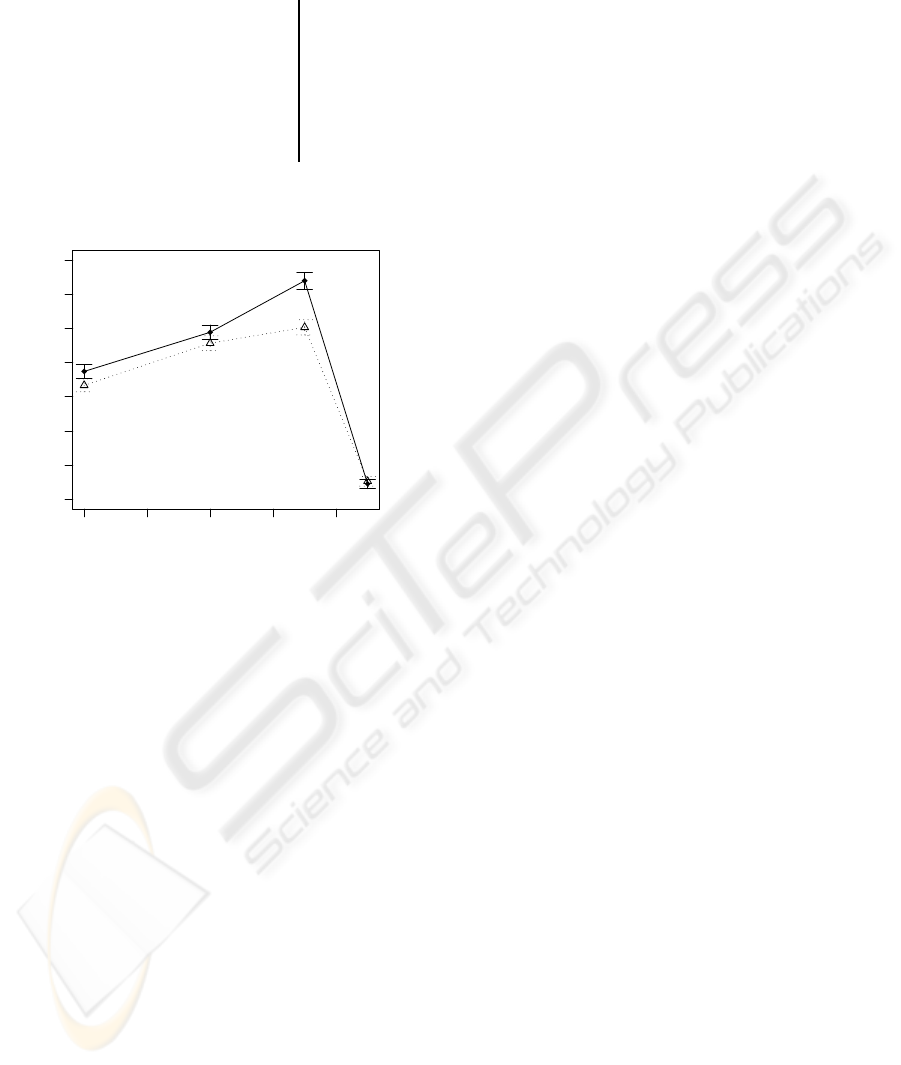
Table 1: Approximate average episode when successful bal-

ancing occurs in different sources, indicated where avail-

able.

This paper 100

(Barto et al., 1983) 80

(Whitehead and Lin, 1995) 200

(Kimura and Kobayashi, 1998) 120

(Schneegaß et al., 2007) 100-150

(Lagoudakis and Parr, 2003) 100

(Mahadevan and Maggioni, 2007) 20

0.0 0.2 0.4 0.6 0.8

20 30 40 50 60 70 80 90

Cart−Pole, RBF

Average Steps/Episode at best α

Figure 8: Average up-time in seconds for Cart-Pole task

with best α value as a function of λ. Error bars indicate one

standard error.

the state space that are actually visited, rather than the

regularly spaced 6×6×6×6 RBF neurons used here,

of which a majority is probably never used. However,

the kernel allocation in (Mahadevan and Maggioni,

2007) requires initial random walks in order to obtain

samples from the task that allow ofﬂine calculation

of corresponding Eigen vectors and allocating ‘Proto-

Value Functions’ from them.

A challenge in interpreting the results of the

experiments performed for this paper is that the

agent ‘un-learns’ after a certain number of success-

ful episodes where no reward signal at all is received.

As pointed out in (Barto et al., 1983), this lack of

reward input slowly deteriorates the already learned

action-value function in critic-only architectures such

as Sarsa(λ). The results shown in Figure 8 include

this phenomenon, i.e. the average values are calcu-

lated for 200 episodes during which the task is suc-

cessfully learned but also possibly un-learned and re-

learned again.

The results shown in Figure 8 differ from those

of the previous tasks by the fact that the accumulat-

ing trace performs slightly better than the replacing

trace and that the parameter sensitivity is quite similar

for both trace types in this task. This difference com-

pared to the two previous tasks is probably due to the

delayed (and rare) reward that allows the eligibility

trace to decline before receiving reward, thus avoid-

ing weight divergence in equation 1. Further empir-

ical results from tasks with delayed reward are still

needed before declaring which eligibility trace type is

better.

5 CONCLUSIONS

Gradient-descent Sarsa(λ) is not a new method for

action-value learning with continuous-valued func-

tion approximation. Therefore it is surprising how lit-

tle empirical knowledge exists that would allow prac-

titioners to assess its usability compared with more

complex RL methods. The only paper of those cited

here that uses gradient-descent Sarsa(λ) is (Santa-

maría et al., 1998). The results obtained in this pa-

per show that at least for the three well-known bench-

mark tests used, gradient-descent Sarsa(λ) together

with NRBF function approximation tends to outper-

form all other methods while being the conceptually

and computationally most simple-to-use method. The

results presented here should provide a useful bench-

mark for future experimentsbecause they seemto out-

perform most previously reported results, even those

where a previously collected training set or a model

of the system dynamics was used directly or learned.

These results are obtained due to the linking of

different pieces together in an operational way. Im-

portant elements are for instance the choice of us-

ing NRBF and the normalisation of state values into

the interval [0,1] that simpliﬁes ﬁnding suitable learn-

ing rates and r

values. The replacing eligibility

trace presented in (Främling, 2007b) is also more sta-

ble against learning parameter variations than the ac-

cumulating trace while giving slightly better perfor-

mance. Future directions of this work could con-

sists in performing experiments with more challeng-

ing tasks in order to see the limits of pure gradient-

descent Sarsa(λ) learning. In tasks where gradient-

descent Sarsa(λ) is not sufﬁcient, combining it with

pre-existing knowledge as in (Främling, 2007a) could

be a solution for applying RL to new real-world con-

trol tasks.

REFERENCES

Abbeel, P., Coates, A., Quigley, M., and Ng, A. Y. (2007).

An application of reinforcement learning to aerobatic

helicopter ﬂight. In Schölkopf, B., Platt, J., and Hoff-

LIGHT-WEIGHT REINFORCEMENT LEARNING WITH FUNCTION APPROXIMATION FOR REAL-LIFE

CONTROL TASKS

133

man, T., editors, Advances in Neural Information Pro-

cessing Systems 19, pages 1–8, Cambridge, MA. MIT

Press.

Abramson, M., Pachowicz, P., and Wechsler, H. (2003).

Competitive reinforcement learning in continuous

control tasks. In Proceedings of the International

Joint Conference on Neural Networks (IJCNN), Port-

land, OR, volume 3, pages 1909–1914.

Albus, J. S. (1975). Data storage in the cerebellar model ar-

ticulation controller (cmac). Journal of Dynamic Sys-

tems, Measurement and Control, September:228–233.

Barto, A., Sutton, R., and Anderson, C. (1983). Neuron-

like adaptive elements that can solve difﬁcult learning

control problems. IEEE Trans. on Systems, Man, and

Cybernetics, 13:835–846.

Doya, K. (2000). Reinforcement learning in continuous

time and space. Neural Computation, 12:219–245.

Främling, K. (2004). Scaled gradient descent learning rate

- reinforcement learning with light-seeking robot. In

Proceedings of ICINCO’2004 conference, 25-28 Au-

gust 2004, Setubal, Spain, pages 3–11.

Främling, K. (2005). Adaptive robot learning in a non-

stationary environment. In Proceedings of the 13

European Symposium on Artiﬁcial Neural Networks,

April 27-29, Bruges, Belgium, pages 381–386.

Främling, K. (2007a). Guiding exploration by pre-existing

knowledge without modifying reward. Neural Net-

works, 20:736–747.

Främling, K. (2007b). Replacing eligibility trace for action-

value learning with function approximation. In Pro-

ceedings of the 15

European Symposium on Artiﬁ-

cial Neural Networks, April 25-27, Bruges, Belgium,

pages 313–318.

Kimura, H. and Kobayashi, S. (1998). An analysis of

actor/critic algorithms using eligibility traces: Rein-

forcement learning with imperfect value functions. In

Proceedings of the 15

Int. Conf. on Machine Learn-

ing, pages 278–286.

Lagoudakis, M. G. and Parr, R. (2003). Least-squares pol-

icy iteration. Journal of Machine Learning Research,

4:1107–1149.

Mahadevan, S. and Maggioni, M. (2007). Proto-value func-

tions: A laplacian framework for learning represen-

tation and control in markov decision processes. J.

Mach. Learn. Res., 8:2169–2231.

Moore, A. (1991). Variable resolution dynamic program-

ming. efﬁciently learning action maps in multivari-

ate real-valued state-spaces. In Machine Learning:

Proceedings of the Eight International Workshop, San

Mateo, CA., pages 333–337. Morgan-Kaufmann.

Santamaría, J., Sutton, R., and Ram, A. (1998). Experi-

ments with reinforcement learning in problems with

continuous state and action spaces. Adaptive Behav-

ior, 6:163–217.

Schaal, S. (1997). Learning from demonstration. In

Advances in Neural Information Processing Systems

(NIPS), volume 9, pages 1040–1046. MIT Press.

Schaefer, A. M., Udluft, S., and Zimmermann, H.-G.

(2007). The recurrent control neural network. In Pro-

ceedings of 15

European Symposium on Artiﬁcial

Neural Networks, Bruges, Belgium, 25-27 April 2007,

pages 319–324. D-Side.

Schneegaß, D., Udluft, S., and Martinetz, T. (2007). Neu-

ral rewards regression for near-optimal policy identi-

ﬁcation in markovian and partial observable environ-

ments. In Proceedings of 15

European Symposium

on Artiﬁcial Neural Networks, Bruges, Belgium, 25-

27 April 2007, pages 301–306. D-Side.

Singh, S. and Sutton, R. (1996). Reinforcement learning

with replacing eligibility traces. Machine Learning,

22:123–158.

Smart, W. D. and Kaelbling, L. P. (2000). Practical rein-

forcement learning in continuous spaces. In Proceed-

ings of the Seventeenth 17

International Conference

on Machine Learning, pages 903–910. Morgan Kauf-

mann.

Strens, M. J. and Moore, A. W. (2002). Policy search us-

ing paired comparisons. Journal of Machine Learning

Research, 3:921–950.

Sutton, R. and Barto, A. (1998). Reinforcement Learning.

MIT Press, Cambridge, MA.

Tesauro, G. (1995). Temporal difference learning and td-

gammon. Communications of the ACM, 38:58–68.

Whitehead, S. and Lin, L.-J. (1995). Reinforcement learn-

ing of non-markov decision processes. Artiﬁcial Intel-

ligence, 73:271–306.

ICINCO 2008 - International Conference on Informatics in Control, Automation and Robotics

134