
ROBOT LOCALIZATION BASED ON VISUAL LANDMARKS
Hala Mousher Ebied, Ulf Witkowski, Ulrich Rückert
System and Circuit Technology, Institute of Heinz Nixdorf, Paderborn Universit
Fürstenallee 11, D-33102 Paderborn, Germany
Mohamed Saied Abdel-Wahab
Department of Scientific Computing, Faculty of Computer and Information Sciences
Ain Shames University, Cairo, Egypt
Keywords: Position system, Vision-based localization, Triangulation, Minirobot, Visual landmarks.
Abstract: In this paper, we will consider the localization problem of the autonomous minirobot Khepera II in a known
environment. Mobile robots must be able to determine their own position to operate successfully in any
environments. Our system combines odometry and a 2-D vision sensor to determine the position of the
robot based on a new triangulation algorithm. The new system uses different colored cylinder landmarks
which are positioned at the corners of the environment. The main aim is to analyze the accuracy and the
robustness in case of noisy data and to obtain an accurate method to estimate the robot’s position.
1 INTRODUCTION
Vision-based localization is the process to recognize
the landmarks reliably and to calculate the robot's
position (Borenstein et al., 1996). Researchers have
developed a variety of systems sensors, and
techniques for mobile robot positioning. (Borenstein
et al., 1997) define seven categories for positioning
system: Odometry, Inertial Navigation, Magnetic
Compasses, Active Beacons (Trilateration method
and Triangulation method), Global Positioning
Systems, Landmark Navigation, and Model
Matching. Some experimental systems that work on
localization are using mobile robots equipped with
sensors that provide range and bearing
measurements to beacons (Witkowski and Rückert,
2002) and some other work with vision sensors
(Chinapirom et al, 2004).
Because of the lack of a single good method,
developers of mobile robots usually combine two or
more methods (Borenstein et al., 1997). To predict
the robot’s location, some systems combine
odometric measurements, landmark matching, and
triangulation with observations of the environment
from a camera sensor (DeSouza and C.Kak, 2002;
Yuen et al., 2005). (Martinelli et al, 2003) combine
the odometric measurements, uses encoder readings
as inputs, and the readings from a laser range finder
as observations to localize the robot.
Many solutions to the localization problem
included geometric calculations which do not
consider uncertainty and statistical solutions (Kose
et al., 2006). Triangulation is a widely used to the
localization problem. It uses geometry data to
compute the robot’s position in indoor environment
(Shoval et al., 1998).
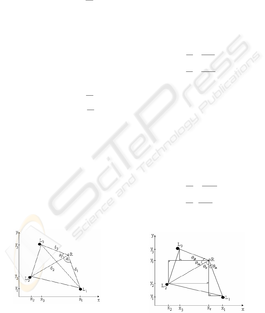
Triangulation is based on the measurement of the
bearings of the robot relatively to the landmarks
placed in known positions. Three landmarks are
required at least for solving the triangulation. The
robot’s position estimated by the triangulation
method is based on find the intersection of the two
circles which passes through the robot and two
landmarks, show figure 1.
Cohen and Koss, 1993 present four methods for
triangulation from three fixed landmarks in known
locations in an environment: iterative search (IS),
geometric triangulation (GT), iterative Newton
Raphson (NR) and geometric circle intersection
(GCI). NR and GCI methods are found to be the
most efficient ones. IS and GT are not practical.
The geometric triangulation method is based on
the law of sins and works consistently only when the
robot is within the triangle formed by the three
49
Mousher Ebied H., Witkowski U., Rückert U. and Saied Abdel-Wahab M. (2008).
ROBOT LOCALIZATION BASED ON VISUAL LANDMARKS.
In Proceedings of the Fifth International Conference on Informatics in Control, Automation and Robotics - RA, pages 49-53
DOI: 10.5220/0001484400490053
Copyright
c
SciTePress
landmarks (Casanova et al., 2002, Esteves et al.,
2003). The geometric circle intersection method is
widely used in literature. It fails when the three
landmarks and the robot lie on a same circle. Betke
and Gurvis, 1997 are using more than three beacons.
The landmark is written as a complex number in
the robot-centered coordinate system. The
processing time depends linearly on the number of
the landmarks. Casanova et al (Casanova et al.,
2002; Casanova et al., 2005) address the localization
problem of moving objects using laser and
radiofrequency technology through a geometric
circle triangulation algorithm. They show that the
localization error varies depending on the angles
between the bacons.
In this paper, a system for global positioning of a
mobile robot is presented. Our system combines
odometry and 2-D vision data to determine the
position of the robot by a new Alternative
Triangulation Algorithm (ATA). ATA is obtained
from a set of equations from the triangles between
the robot and the landmarks. We present simulation
results for noisy input data to estimate the robot’s
position with respect to the environment.
In the next section, the robot platform is
described. Section 3 describes the triangulation
method based on the law of cosine. Section 4
contains the description of the new Alternative
Triangulation Algorithm. Results are given in
section 5.
Figure 1: The robot’s position is the intersection of two
circles. Each one of the two circle passes through the robot
and two landmarks.
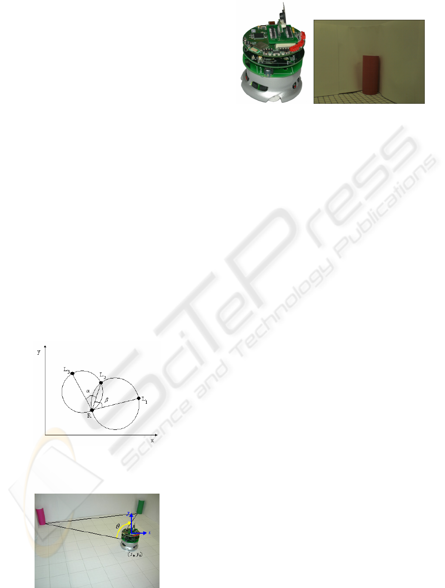
Figure 2: Khepera with the camera module in the test
environment.
Figure 3: Khepera minirobot II equipped with FPGA
module and 2D color CMOS camera module, and a typical
image with 640 x 480 pixels from camera module.
2 ROBOT PLATFORM
The main idea is the detection of landmarks of
different color by using a CMOS color sensor. For
this, the robot gets pictures of the environment in
different orientations and/or from different positions.
An image processing algorithm will be used to
extract the centre of each landmark; details are given
in (Ebied et al., 2007). Also the different angles
between different landmarks as viewed from the
mobile robot will be calculated using the odometry
method as show in figure 2. Then we develop a new
alternative triangulation algorithm to calculate the
robot’s position based on parameter set (angles) and
the knowledge of the positions of the landmarks.
The positioning system has been implemented on
the minirobot Khepera (K-Team, 2002) that uses an
additional camera module, as show in figure 2. The
camera is a 2D color CMOS camera from Transchip,
model TC5740MB24B. To control the camera we
use an FPGA module that is equipped with USB 2.0
port. Via the USB port the programmer is able to see
on a computer screen what the robot is capturing.
The received images have a resolution of 640 x 480
pixels in 8 bit RGB color, see figure 3.
3 THE TRIANGULATION
ALGORITHM
This section shows how to apply well-known
triangulation algorithm (Betke and Gurvis, 1997) to
the robot localization problem. If the positions of the
landmarks are known and also the angles between
the landmarks relative to the robot’s position are
known, then we can use the law of cosine to
calculate the distance between the robot and the
three landmarks. Let (x
i
,y
i
), i=1…3 be the positions
of the landmarks L
1
… L
3
in the Cartesian
ICINCO 2008 - International Conference on Informatics in Control, Automation and Robotics
50
coordinate of the environment. From the triangle
between the robot and the landmarks L
1
and L
2
, we
get the following equation by applying the law of
cosine
()
()
180
1
cos
21
2
2
2
2
1
2
21
π
θddddxx ∗−+=−
(1)
where d
i
, i=1…3 are the unknown distance
between the landmarks and the robot’s position, and
θ
1
is the angle between landmarks L
1
and L
2
relative
to the robot’ position, as shows in figure 4.
With three landmarks, there are three pairs of
landmarks (i.e. landmarks 1 and 2, 2 and 3, and 1
and 3). So we can get system of equations to
determine the distance d
i
between the robot’s
position and the landmarks L
i
, by applying the law
of cosine to all pairs of landmarks
()
(
)
180
2
cos
31
2
2
3
2
1
2
31
π
θ
∗−+=− ddddxx
(2)
()
()
180
12
cos
32
2
2
3
2
2
2
32
π
θ
∗−+=− ddddxx
(3)
Where θ
2
is the angle between landmarks L
2
and
L
3
relative to the robot’ position, as shown in figure
4. The system of nonlinear equations (1), (2), and (3)
can be solved using a least square method. Once the
distances d
i
are found, the robot’s position (x
r
,y
r
)
can be estimated from solving the following
equations:
()()
2
1
2
1
2
1
r
yy
r
xxd −+−=
(4)
()()
2
2
2
2
2
2
r
yy
r
xxd −+−=
(5)
()()
2
3
2
3
2
3 r
yy
r
xxd −+−=
(6)
Figure 4: Estimated robot’s position R using law of cosine.
4 AN ALTERNATIVE
TRIANGULATION
ALGORITHM
In the alternative triangulation algorithm, also at
least three landmarks are required to estimate the
robot’s position. We can use the triangles between
the robot and the three landmarks to estimate the
robot’s position. From the triangle between the robot
and the landmarks L
1
and L
2
, we get the following
equations
(
)
()
2
2
180
*
1
tan
1
1
180
*
1
tan
y
r
y
x
r
x
b
y
r
y
r
xx
a
−
−
=
−
−
=
π
θ
π
θ
(7)
(8)
The angles θ
1a
and θ
1b
can be computed from the
measured angle θ
1
, as shows in figure 5.
111
θθθ
=+
ba
(9)
We can apply the same equations to another pair of
landmarks and get a system of six equations in six
unknown variables which can be solved to give us
an estimate for the robot’s position (x
r
, y
r
). Applying
the same equations on the triangle between the robot
and the landmarks L
2
and L
3
, we get the following
equations
(
)
()
222
3
3
180
*
2
tan
2
2
180
*
2
tan
θθθ
π
θ
π
θ
=+
−
−
=
−
−
=
ba
x
r
x
r
yy
b
x
r
x
y
r
y
a
(10)
(11)
(12)
Figure 5: An alternative triangulation algorithm to
estimated robot’s position R using three Landmarks.
ROBOT LOCALIZATION BASED ON VISUAL LANDMARKS
51
5 RESULTS AND DISCUSSION
Four distinctly coloured landmarks are placed at
known positions at the edges of the environment.
For a robot’s environment with a size of 62 x 74
cm
2
, the floor of the environment will be divided
into squares (cells) that are used to determine the
position of the robot. We have used a grid with 11
by 13 lines in each direction which results in a data
set of 143 robot’s position. The robot’s position
error is considering as the Euclidean distance
between the estimated robot position and the actual
robot position. We averaged the robot’s position
error over 143 places in the environment.
In the first experiment, the alternative
triangulation algorithm has been used to estimate
robot’s position in the experimental environment.
The experiments deal with different combinations of
three landmarks. In Figure 6, the position error has
been plotted as a function of the robot’s position.
The average of the position error is 0.35cm which is
limited between 0.02cm and 3.5cm. Maximum error
is obtained when the two angles between three
landmarks relative to the robot’s position is less than
90
○
. It is easily to overcome the error in robot’s
position by using all the visible landmarks.
Using several landmarks yield a more robust
robot’s position estimate. If we have n landmarks,
there are many different combinations of the three
landmarks that can be used to compute the position
of the robot. We can obtain the minimum position
error by using two different ways. First, we can
calculate the average from the estimated robot’s
position from all different groups of three
landmarks. Or by using a suitable algorithm to select
the best 3 landmarks with at least one angle greater
than 90
○
.
The position error average from all different
groups of landmarks is 0.253cm which is limited
between 0.022cm and 0.935cm. The position error,
based on selecting the best 3 landmarks with at least
one angle greater than 90
○
, is 0.242cm which is
limited between 0.021cm and 0.767cm. So by using
a suitable algorithm to select the best 3 landmarks
with at least one angle greater than 90
○
, we can
obtain the minimum position error, as show in figure
7.
The second experiment deals with the
triangulation algorithm based on the law of cosine.
Solving system of nonlinear equations using the
least square method requires making a starting guess
of the robot’s position. Table 1 shows the results of
the experiments in which the starting guess of the
solution takes across the environment diagonal. Our
results show the minimum, maximum, mean, and
standard deviation of the position error. We begin to
receive a minimum of the position error close to the
environment center. The mean of the position error
is 0.0035cm when the center coordinate of the
environment is used as the starting guess.
The last experiment, we consider the robot’s
position problem for noisy angle data that are
measure using odometry method. Errors in odometry
are caused by the intersection between the wheels
and the terrain, for example slippage, cracks, debris
of solid material, etc. (Borenstein et al., 1997). We
add a random noisy angle
θ
Δ
of degree to each
actual angle. Table 2 shows the position error using
the alternative triangulation algorithm with different
combinations of three landmarks, and using the
random generated angles
θ
Δ
on the specified
interval [-3
○
, 3
○
]
which are added to the actual
angles.
Figure 6: Estimated robot’s position using an ATA. Three
landmarks have been placed at the right and left bottom
corner and at the left top corner of the environment. The
maximum error happened when the robot was been almost
on the same line with one of the landmarks parallel to the
x-axis.
Figure 7: By using a suitable algorithm to select the best 3
landmarks with at least one angle greater than 90
○
.
ICINCO 2008 - International Conference on Informatics in Control, Automation and Robotics
52
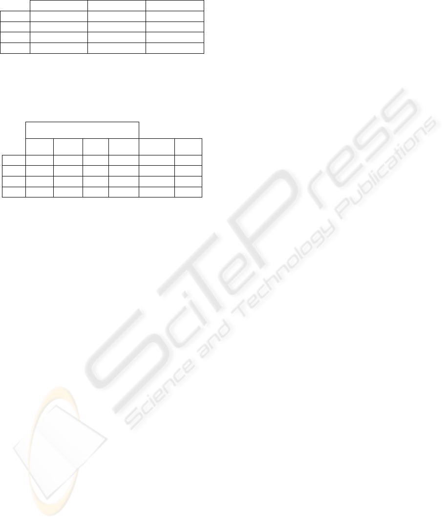
Table 1: Minimum, maximum, mean, and standard
deviation values (in cm) for the robot’s position error at
different starting guess of the solution.
(10,10,10)cm (15,15,15)cm (20,20,20)cm
min 0,0002 0,0002 0,0002
max 66,0609 66,0609 0,0351
mean 8,0755 1,8593 0,0035
std 18,1959 10,5717 0,0046
Table 2: Minimum, maximum, mean, and standard
deviation values (in cm) for the robot’s position error of
different groups of landmarks. The results from selecting
the suitable three landmarks with at least one angle greater
than 90
○
are given in column Select.
Landmark groups
1, 2, 3 1, 2, 4 2, 3, 4 1, 3, 4 average Select
m
in 0,222 0,102 0,097 0,047 0,106 0,20
m
ax 8,631 10,12 11,01 21,24 6,490 4,07
m
ean 1,924 1,944 2,136 2,154 1,403 1,50
St
d
1,511 1,602 2,065 2,520 0,897 0,88
ACKNOWLEDGEMENTS
This work is a result of common research between
the Department of System and Circuit Technology,
Heinz Nixdorf Institute, University of Paderborn and
Scientific Computing Department, Faculty of
Computer and Information Sciences, Ain Shames
University. It is also supported from the Arab
Republic of Egypt cultural department and study
mission.
REFERENCES
Betke, M., and Gurvits, L., 1997. Mobile Robot
Localization Using Landmarks. IEEE Transactions On
Robotics And Automation, Vol. 13, No. 2.
Borenstein, J., Everett, H. R. and Feng, L., 1996. Where
am I? Sensors and Methods for Mobile Robot
Positioning, Technical Report, The University of
Michigan.
Borenstein J., Everett, H. R., Feng, L., and Wehe, D.,
1997. Mobile Robot Positioning: Sensors and
Techniques, Journal of Robotic Systems, vol. 14, , pp.
231-249.
Casanova, E. Z., Quijada, S. D., García-Bermejo, J. G.,
and González, J. R. P., 2002. A new beacon based
system for the localisation of moving objects. 9th
IEEE International Conference on Mechatronics and
Machine Vision in Practice, pp. 59-64, Chiang Mai,
Tailandia.
Casanova, E. Z., Quijada, S. D., García-Bermejo, J. G.,
and González, J. R. P., 2005. Microcontroller based
System for 2D Localisation , Mechatronics, Vol. 15,
Issue 9, pp. 1109-1126.
Chinapirom, T., Kaulmann, T., Witkowski, U., and
Rückert, U., 2004. Visual Object Recognition by 2d-
Color Camera and On-Board Information Processing
For Minirobots. FIRA Robot World Congress Busan,
South Korea.
Cohen, C. and Koss, F., 1993. A Comprehensive Study of
Three Object Triangulation. SPIE Conference on
Mobile Robots, Boston, MA, pp. 95-106.
DeSouza, G.N., and C.Kak, A., 2002. Vision for Mobile
Robot Navigation:ASurvey. IEEE Transactions on
pattern analysis and Machine intelligence, Vol. 24,
No.2.
Ebied, H. M., Witkowski, U., Rückert, U., and Abdel-
Wahab, M. S., 2007. Robot Localization System
Based on 2D-Color Vision Sensor, 4
th
International
Symposium on Autonomous Minirobots for Research
and Edutainment, pp. 141-150, Buenos Aires,
Argentina.
Esteves, J.S., Carvalho, A., Couto, C., 2003. Generalized
Geometric Triangulation Algorithm for Mobile Robot
Absolute Self-Localization. IEEE International
Symposium on Industrial Electronics, pp. 346 – 351.
Kose, H., Celik, B., and Levent Akın, H., 2006.
Comparison of Localization Methods for a Robot
Soccer Team, International Journal on Advanced
Robotic Systems, Vol. 3, No. 4, pp. 295-302.
K-Team, S.A. 2002. Khepera 2 User Manual. Ver 1.1,
Lasanne, Switzerland.
Martinelli, A., Tomatis, N., Tapus, A., and Siegwart, R.,
2003. Simultaneous Localization and Odometry
Calibration for Mobile Robot. IEEE International
Conference on Intelligent Robots and Systems, pp.
1499-1504, Las Vegas, Nevada.
Shoval, S., Mishan, A., and Dayan, J., 1998. Odometry
and Triangulation Data Fusion for Mobile-Robots
Environment Recognition, International Journal on
Control Engineering Practice, Vol. 6, Issue 11, pp.
1383-1388.
Witkowski, U., and Rückert, U., 2002. Positioning
System for the Minirobot Khepera based on Self-
organizing Feature Maps. FIRA Robot World
Congress, pp. 463-468, COEX, Seoul, Korea.
Wolf, J., Burgard, W. and Burkhardt, H., 2005. Robust
Vision-Based Localization by Combining an Image-
Retrieval System with Monte Carlo Localization.
IEEE Transactions on Robotics, Vol. 21, No. 2, pp.
208-216.
Yuen, D. C. K., and MacDonald, B. A., 2005. Vision-
Based Localization Algorithm Based on Landmark
Matching, Triangulation, Reconstruction, and
Comparison, IEEE Transactions On Robotics, Vol. 21,
No. 2, pp. 217-226.
ROBOT LOCALIZATION BASED ON VISUAL LANDMARKS
53
