EXPONENTIAL OBSERVER FOR A CLASS OF NONLINEAR
DISTRIBUTED PARAMETER SYSTEMS WITH APPLICATION TO
A NONISOTHERMAL TUBULAR REACTOR
Nadia Barje, Mohammed Achhab
Laboratoire d’Ing´enierie Mathematique (LINMA), Universit´e Chouaib Doukkali, El Jadida, Morroco
Vincent Wertz
∗
CESAME, Universit de Louvain, Louvain-la-Neuve, Belgium
Keywords:
Nonlinear infinite-dimensional systems, state observer, nonlinear tubular reactor.
Abstract:
This paper present sufficient conditions to construct an exponential state estimator for a class of infinite dimen-
sional non-linear systems driven in a real Hilbert state description. The theory is applied to a nonisothermal
plug flow tubular reactor, governed by hyperbolic first order partial differential equations. For this application
performance issues of the exponential state estimator design are illustrated in a simulation study.
1 INTRODUCTION
State estimators for dynamical systems have been
the focus of an intensive work in the last decades.
The classical theory of the Luenberger observers has
been successfully extended from finite dimensional
linear systems to a large class of infinite dimensional
linear systems by many authors, since the pioneer-
ing paper by (Gressang and Lamont, 1975). Later,
the theory has been generalized to a class of sin-
gle input distributed bilinear systems in (Gauthier
et al., 1995). The paper of (Bounit and Hammouri,
1997) consider a class of distributed bilinear systems
witch are observable for ”small inputs” and gives a
strong exponential observer. Recently, for nonlinear
models of non-isothermal tubular reactors considered
in (Laabissi et al., 2001), the paper of (Orlov and
Dochain, 2002) presented a reduced-order observer
of the concentration, assuming that the temperature
is the only available measurement.
The primary objective of this paper is to address the
problem of the design of exponential Luenberger-like
observers for a class of infinite dimensional nonlinear
∗
This work was finalized when this author was on sab-
batical leave at the ARC Centre of Excellence for Complex
Dynamic Systems and Control, The University of Newcas-
tle, Australia, whose support is gratefully acknowledged.
systems described by the following equation

˙x(t) = Ax(t) + N(x(t)), x(0) ∈ D(A) ∩ D
y(t) = Cx(t)
(1)
Here, A is the infinitesimal generator of a C
0
-
semigroup on a real Hilbert space H with inner prod-
uct < ., . > and norm k . k, D(A) is the domain of A,
N is a nonlinear operator from a closed subset D of
H into H, y(t) ∈ Y is the known output function as-
sociated to the unknown initial condition x(0), Y is
another real Hilbert space and C is a bounded linear
operator from H into the Hilbert space Y. Under the
assumption that N is locally Lipschitz continuous, it
is shown in ((Pazy, 1983), pp. 185-186) that equa-
tion (1) has a unique mild solution on some interval
[0,t
max
), t
max
∈ (0,+∞] given by

x(t) = S(t)x(0) +
R
t
0
S(t − s)N(x(s))ds,
0 ≤ t < t
max
(2)
where (S(t))
t≥0
denotes theC
0
−semigroup generated
by A. To ensure that the problem is well posed,
we shall assume throughout the paper as in (Laabissi
et al., 2001) that we have: t
max
= +∞. An observer
design is presented for which a result about the expo-
nential convergence of the estimation error is stated
under verifiable conditions.
Our second objective is to apply the previous devel-
oped result to the nonlinear model of a chemical plug
flow reactor. This model is showed to be described
20
Barje N., Achhab M. and Wertz V. (2008).
EXPONENTIAL OBSERVER FOR A CLASS OF NONLINEAR DISTRIBUTED PARAMETER SYSTEMS WITH APPLICATION TO A NONISOTHERMAL
TUBULAR REACTOR.
In Proceedings of the Fifth International Conference on Informatics in Control, Automation and Robotics - ICSO, pages 20-27
DOI: 10.5220/0001484900200027
Copyright
c
 SciTePress

by (1). Trajectory analysis of such a model of chem-
ical plug flow reactors has been done extensively in
(Achhab et al., 1999) and (Laabissi et al., 2001). For
this application, we also introduce a second observer
in the case when only one of the two states, namely
the temperature, is measured and show the exponen-
tial convergenceof both estimation errors. A third ob-
server is then introduced to improve the convergence
rate of the previous one. Simulations results are then
presented in order to highlight the performance issues
of the proposed observers.
The paper is organized as follows. In section 2, we
consider a general observer design for system (1).
Then, we state sufficient conditions under which the
related estimation error converges exponentially to
zero. The approach developed in the general setting
is applied to a chemical plug flow reactor model in
section 3. In section 4, simulation results are given in
order to illustrate some performance issues of this ap-
plication. Finally, the paper closes with some remarks
and conclusions in section 5. The background of the
approach is to be found in (Curtain and Zwart, 1995)
and (Cazenave and Haraux, 1998).
2 OBSERVER DESIGN
We state in this section sufficient conditions under
which we will be able to show that the estimation
error of the Luenberger-like observer converges
exponentially to zero.
Let us assume that the following.
A.1. The linear operator A satisfies for all x ∈ D(A),
and t ≥ 0, < Ax(t),x(t) >≤ 0.
A.2. The nonlinear operator N is a k
N
-Lipschitz oper-
ator on its domain D, where k
N
is a positive constant;
i.e. for all x,y ∈ D, k N(x) − N(y) k≤ k
N
k x− y k.
A.3. The pair (A,C) is approximately observable
linear system (i.e. ∀e ∈ H, {CS(t)e = 0, ∀t ≥
0, implies e = 0}), exponentially stable.
A.4. The semigroup S(.) satisfies for all e ∈ H:
< S
∗
(.)C
∗
CS(.)e,e >≤k S(.) k
2
< C
∗
Ce,e >,
Comment 2
.1. The hypothesis A.3 implies that the
linear system

˙x(t) = Ax(t), x(0) ∈ D(A)
y(t) = Cx(t)
is approximately observable on [0,+∞) and that the
observability gramian L
C
:=C
∗
C, whereCe := CS(.)e
for all e ∈ H, and C
∗
is the adjoint of the linear op-
erator C, is bounded positive definite (see (Curtain
and Zwart, 1995), p.160), and thus has an algebraic
bounded inverse with domain equal to range L
C
.
Consider now the following candidate observer

˙
ˆx(t) = Aˆx(t) + N( ˆx(t)) − GC
∗
(C ˆx(t) − y(t))
ˆx(0) ∈ D(A) ∩ D
(3)
where G is a linear bounded operator and y(t) is
the known output function of the system (1). One
can show that system (3) admits a unique solution
ˆx(t) which is well defined for any initial condition
ˆx(0) ∈ D(A) ∩ D and for all t ∈ [0,t
max
), with t
max
as-
sumed to be equal +∞.
Setting e(t) = x(t)− ˆx(t), the reconstruction error e(t)
obeys the following equation:
˙e(t) = Ae(t) + N(x(t)) − N( ˆx(t)) − GC
∗
Ce(t) (4)
and one obtains the following theorem:
Theorem 2.1
. Let assumptions A.1-A.4 be satisfied. If
there exists a bounded linear operator G and a posi-
tive real number g such that g > k
N
and for e ∈ H, e 6=
0,
< GC
∗
Ce,e > ≥ < g k L
−1
C
kk S(.) k
2
C
∗
Ce,e >
then, system (3) is an exponential observer for system
(1). More precisely, the reconstruction error satisfies
k e(t) k
2
≤k e(0) k
2
e
−ηt
where η = 2(g − k
N
).
Proof 2.1
. The computation of the derivative of the
functional
V
e
(t) =
1
2
k e(t) k
2
along the trajectories of (4) yields,
˙
V
e
(t) =< ˙e(t),e(t) >
=< Ae(t),e(t) > + < N(x(t)) − N(ˆx(t)),e(t) >
− < GC
∗
Ce(t),e(t) >
and in addition,
< GC
∗
Ce,e > ≥ g k L
−1
C
kk S(.) k
2
< C
∗
Ce,e >
≥ g k L
−1
C
k< L
C
e,e >
≥ g < e,e >
indeed, the operator L
C
is self-adjoint and nonnega-
tive (i.e, < L
C
e,e >≥ 0 for all e ∈ H), then L
C
has a
unique square root L
1
2
C
self-adjoint, so that L
1
2
C
L
1
2
C
e =
L
C
e for all e ∈ H (see (Curtain and Zwart, 1995),
p.606), the operator L
−1
C
is also self-adjoint and non-
negative, par consequent has a unique square root
(L
−1
C
)
1
2
= (L
1
2
C
)
−1
(see (Curtain and Zwart, 1995), pp.
603-610).
and in addition, for all e ∈ H,
< L
−1
C
e,e > ≤k L
−1
C
k< e,e >
EXPONENTIAL OBSERVER FOR A CLASS OF NONLINEAR DISTRIBUTED PARAMETER SYSTEMS WITH
APPLICATION TO A NONISOTHERMAL TUBULAR REACTOR
21

thus,
k L
−1
C
k< L
C
e,e > =k L
−1
C
k< L
1
2
C
L
1
2
C
e,e >
=k L
−1
C
k< L
1
2
C
e,L
1
2
C
e >
≥< L
−1
C
L
1
2
C
e,L
1
2
C
e >
≥< (L
1
2
C
)
−1
L
1
2
C
e,(L
1
2
C
)
−1
L
1
2
C
e >
=< e,e >
Hence,
˙
V
e
(t) ≤k N(x(t)) − N( ˆx(t)) kk e(t) k −g k e(t) k
2
≤ (k
N
− g) k e(t) k
2
= −ηV
e
(t)
Now, using Gronwall’s Lemma (see (Curtain and
Zwart, 1995), p. 639), we get
V
e
(t) ≤ V
e
(0)e
−ηt
Consequently, one may deduce
k e(t) k
2
≤k e(0) k
2
e
−ηt
This shows the exponential convergence of the esti-
mation error and the proof of Theorem (2.1) is thus
complete.
2.1 Application to a Nonisothermal
Plug-Flow Reactor
The theory developed in the general setting is applied
to a chemical non-isothermal tubular reactor with the
following chemical reaction:
A → B
The kinetics of the above reaction is characterized by
first-order kinetics with respect to the reactant con-
centration C(mol/l) and by an Arrhenius-type depen-
dence with respect to the temperature T(K), and the
dynamics of the process are described by the follow-
ing two energy and mass balance PDEs (see (Laabissi
et al., 2001)):
∂T
∂τ
= −υ
∂T
∂ζ
−
4h
ρC
p
d
(T − T
c
) −
∆H
ρC
p
k
0
Ce
−E
RT
, (5)
∂C
∂τ
= −υ
∂C
∂ζ
− k
0
Ce
−E
RT
, (6)
where the boundary conditions are given, for τ ≥ 0,
by:
T(0, τ) = T
in
, C(0, τ) = C
in
(7)
and the initial conditions are assumed to be given, for
0 ≤ ζ ≤ L, by:
T(ζ, 0) = T
0
(ζ), C(ζ,0) = C
0
(ζ) (8)
In the equations above, the following parameters
υ, ∆H, ρ, C
p
, k
0
, E, R, h, d, T
c
hold for the super-
ficial fluid velocity, the heat of reaction, the density,
the specific heat, the kinetic constant, the activation
energy, the ideal gas constant, the wall heat transfer
coefficient, the reactor diameter, the coolant temper-
ature. T
in
and C
in
are respectively the inlet temper-
ature and the inlet reactant concentration which will
be assumed to be two positive constants. τ,ζ and L
denote the time and space independent variables, and
the length of the reactor, respectively. Finally T
0
and
C
0
denote the initial temperature and reactant concen-
tration profiles.
The dynamics will be described by means of an
infinite-dimensional system derived from an equiva-
lent nonlinear PDE dimensionless model. Such an
approach is standard in tubular reactor analysis (see
(Laabissi et al., 2001)) and is briefly developed here.
Let here after H = L
2
[0,L] ×L
2
[0,L], endowed by the
inner product
< (x
1
,x
2
),(y
1
,y
2
) >=< x
1
,y
1
>
L
2
+ < x
2
,y
2
>
L
2
and the induced norm
k (x
1
,x
2
) k= (k x
1
k
2
L
2
+ k x
2
k
2
L
2
)
1
2
for all (x
1
,x
2
) and (y
1
,y
2
) in H. We will denote here
after <,>
L
2
by <,>.
Consider the following dimensionless state variables:
x
1
=
T − T
in
T
in
, x
c
=
T
c
− T
in
T
in
,
x
2
=
C
in
−C
C
in
, r(x
1
) = e
µx
1
1+x
1
Let us consider also dimensionless time t and space z
variables:
t =
τυ
L
, z =
ζ
L
.
We shall assume in the rest of the paper that the
coolant temperature T
c
is equal to the inlet temper-
ature T
in
( i.e x
c
≡ 0), since x
c
will be eliminated in
the equation of the reconstruction error between the
plan state and the observer state.
Then we obtain the following equivalent representa-
tion of the model (5)-(8):
∂x
1
∂t
= −
∂x
1
∂z
− βx
1
+ αδ(1− x
2
)r(x
1
) (9)
∂x
2
∂t
= −
∂x
2
∂z
+ α(1− x
2
)r(x
1
) (10)
with the boundary conditions:
x
1
(z = 0,t) = 0, x
2
(z = 0,t) = 0 (11)
ICINCO 2008 - International Conference on Informatics in Control, Automation and Robotics
22

and initial conditions
x
1
(z,0) = x
0
1
, x
2
(z,0) = x
0
2
(12)
and the parameters α, β, δ and µ are related to the
original parameters as follows:
µ =
E
RT
in
, α =
k
0
L
υ
exp(−µ)
β =
4hL
ρC
p
dυ
, δ = −
∆H
ρC
p
C
in
T
in
.
From a physical point of view it is expected that for all
z ∈ [0, 1], and for all t ≥ 0 (see (Aksikas et al., 2007)),
0 ≤ T(z,t) ≤ T
max
and 0 ≤ C(z,t) ≤ C
in
or equivalently
−1 ≤ x
1
(z,t) ≤
T
max
− T
in
T
in
and 0 ≤ x
2
(z,t) ≤ 1,
where T
max
could possibly be equal to +∞.
This is also true for the model, as shown by (Laabissi
et al., 2001).
The equivalent state space description of the model
(9)-(12) is given by the following nonlinear ab-
stract differential equation on the Hilbert space H =
L
2
[0,1] × L
2
[0,1]:

˙x(t) = Ax(t) + N(x(t))
x(0) = x
0
∈ D(A) ∩ D
(13)
where, A is the linear operator defined on its domain
D(A) := {x =

x
1
x
2

T
∈ H : x absolutely
continuous,
dx
dz
∈ H and x
i
(0) = 0,i = 1,2}
by,
Ax :=

A
1
0
0 A
2

x
1
x
2

=

−
d.
dz
− β. 0
0 −
d.
dz

x
1
x
2

The linear operator A satisfies,
< Ax,x >≤ −
1
2
x
2
(1), for all x ∈ D(A)
which satisfies the hypothesis A.1.
A is the generator of a C
0
-semigroup exponentially
stable
S(t) =

S
1
(t) 0
0 S
2
(t)

satisfying (see (Winkin et al., 2000)), for all (x
1
,x
2
) ∈
H,
(S
1
(t)x
1
)(z) =

e
−βt
x
1
(z−t) if z ≥ t,
0 if z < t,
(S
2
(t)x
2
)(z) =

x
2
(z−t) if z ≥ t,
0 if z < t,
Moreover, (see (Winkin et al., 2000))
k S(t) k ≤ 1 for all t ≥ 0
The nonlinear operator N is defined on
D := {x =

x
1
x
2

T
∈ H : −1 ≤ x
1
(z) and
0 ≤ x
2
(z) ≤ 1, for almost all z ∈ [0,1]} by,
N(x) = (N
1
(x),N
2
(x))
T
where for all x = (x
1
,x
2
)
T
∈
D,
N
1
(x) = αδ(1− x
2
)r(x
1
)
N
2
(x) = α(1− x
2
)r(x
1
)
It is proved in (Aksikas et al., 2007) that the function
m(s) := exp(
−k
s
) where k =
E
R
, is a Lipschitz contin-
uous function on [0,T
max
] with a Lipschitz constant l
s
given by
l
s
=



4
R
Ee
2
if E ≤ 2RT
max
E
RT
2
max
exp(−
E
RT
max
) if E > 2RT
max
It follows that the constant k
r
:= e
µ
T
in
l
s
is a Lipschitz
constant for the function r(s) := exp(
µs
1+s
).
We prove that for all
x := (x
1
,x
2
)
T
and y := (y
1
,y
2
)
T
∈ D,
k N
2
(x) − N
2
(y) k ≤ αexp(µ) k x
2
− y
2
k
+αk
r
k x
1
− y
1
k,
Observe that N
1
= δN
2
, thus we take k
N
:=
α(exp(µ) + k
r
)(1+ | δ |) as a Lipschitz constant of N,
the hypothesis A. 2 is thus satisfied.
It is proved in (Laabissi et al., 2001) that the system
Eq. 13 has a unique mild solution x(t,x(t = 0)) on
[0,+∞[, for all x
0
∈ D and that the state remains in D.
Hereafter we consider measurements at the reactor
output. In this case, the output function y(.) is defined
as follows: we consider a (very small) finite interval
at the reactor output [1− w,1] such that:
y(t) = (Cx)(t) :=
Z
1
0
X
[1−w,1]
(a)I
2×2
x(a,t)da, ∀t ∈ R
+
where
X
[1−w,1]
(a) =

1, if a ∈ [1− w,1]
0, elsewhere.
and I
2×2
is either the 2 × 2 identity matrix operator
when both components x
1
and x
2
are measured, or a
unit row vector if only one of them is measured. In
the first case (i.e. two measurements), it is proved
EXPONENTIAL OBSERVER FOR A CLASS OF NONLINEAR DISTRIBUTED PARAMETER SYSTEMS WITH
APPLICATION TO A NONISOTHERMAL TUBULAR REACTOR
23

in (Winkin et al., 2000), that the pair (C,A) is ap-
proximately observable if both x
1
and x
2
are mea-
sured at the reactor output, thus hypothesis A.3 is
satisfied and so the observability gramian L
C
:= C
∗
C,
where Cx := CS(.)x for all x ∈ H is positive definite
and has an algebraic inverse L
−1
C
with domain equal
to range L
C
, satisfying for x
d
(z,t) = I
d
(z,t), where
I
d
(z,t) = 1 for all (z,t) ∈ [0,1] × R
+
:
< L
C
x
d
,x
d
> =< CS(.)x
d
,CS(.)x
d
>
≥ w
2
e
−2β
k x
d
(z) k
2
on have
k L
C
k
2
≥ w
2
e
−2β
k L
C
k
and
< L
C
x,L
C
x >≥ w
2
e
−2β
< L
C
x,x >
Observe that L
C
is self-adjoint and for all y ∈
range L
C
,
< L
−1
C
y,y > =< L
−1
C
y,L
C
L
−1
C
y >
≤
1
w
2
e
−2β
< L
C
L
−1
C
y,L
C
L
−1
C
y >
≤
1
w
2
e
−2β
< y,y >
this implies,
k L
−1
C
k≤
1
w
2
e
−2β
Denote w
0
= w
2
e
−2β
A candidate Luenberger-observer for system (9)-(12)
when the state variables are measured is
∂ˆx
1
∂t
= −
∂ˆx
1
∂z
− βˆx
1
+ αδ(1− ˆx
2
)r( ˆx
1
) +
g
w
0
C
∗
1
C
1
e
1
(14)
∂ˆx
2
∂t
= −
∂ˆx
2
∂z
+ α(1− ˆx
2
)r( ˆx
1
) +
g
w
0
C
∗
2
C
2
e
2
(15)
with the boundary conditions:
ˆx
1
(z = 0,t) = 0, ˆx
2
(z = 0,t) = 0 (16)
and initial conditions
ˆx
1
(z,t = 0) = ˆx
0
1
, ˆx
2
(z,t = 0) = ˆx
0
2
(17)
with C =

C
1
C
2

and e
i
(z,t) = x
i
(z,t) − ˆx
i
(z,t)
for i = 1, 2, for all (z,t) ∈ [0,1] × R
+
.
The observer state remains in the set D, the main steps
of the proof go along the line of the one given in
(Laabissi et al., 2001).
Observe that the model (14)-(17) is in the form of the
nonlinear abstract differential equation (3), with the
linear operator G chosen as follows: G =
g
w
0
I where I
is the identity operator and g is a positive real number.
For the bounded operator C given above,
the C
0
−semigroup (S(t))
t≥0
satisfies for all e =
(e
1
,e
2
)
T
∈ H:
< S(.)C
∗
CS(.)e,e > ≤k S(.) k
2
< C
∗
Ce,e >
which satisfies the hypothesis A.4.
Denote e(t) the reconstruction error between the plant
state and the observer state. A direct application of
Theorem 2.1 yields the following result.
Corollaire 2.1
. Take g such that g > k
N
holds. Then,
system (14)-(17) is an exponential observer for system
(9)-(12). More precisely, the reconstruction error e(t)
has the property that k e(t) k
2
≤k e(0) k
2
e
−ηt
, where
η = 2(g− k
N
).
It is also interesting to examine the case where only
the temperature x
1
(z,t) is measured at the output
of the reactor. So, the observation operator C =

C
1
C
2

is given by
(C
1
e
1
)(t) =
R
1
0
X
[1−w,1]
(a)e
1
(a,t)da, ∀t ∈ R
+
C
2
= 0
Recall that the linear operator A is diagonal. The op-
erators A
1
and A
2
satisfy;
< A
i
x
i
,x
i
>≤ −
1
2
x
2
i
(1), for all x
i
∈ D(A
i
) and i = 1,2
on their common domain:
D(A
i=1,2
) = {x ∈ L
2
[0,1] : xabsolutely continuous,
dx
dz
∈ L
2
[0,1] and x(0) = 0}.
In the same manner as in (see (Winkin et al., 2000)),
we prove that (C
1
,A
1
) is approximately observable.
In this case, a full-order observer for the dimension-
less model (9)-(12) can be constructed as follows:
∂ˆx
1
∂t
= −
∂ˆx
1
∂z
− βˆx
1
+ αδsup
x
2
∈D
2
(1− x
2
)r( ˆx
1
) +
g
w
0
C
∗
1
C
1
e
1
(18)
∂ˆx
2
∂t
= −
∂ˆx
2
∂z
+ α(1− ˆx
2
)sup
x
1
∈D
1
r(x
1
) (19)
with the boundary conditions:
ˆx
1
(z = 0,t) = 0, ˆx
2
(z = 0,t) = 0 (20)
and initial conditions
ˆx
1
(z,t = 0) = ˆx
0
1
, ˆx
2
(z,t = 0) = ˆx
0
2
(21)
Note that in this observer, the nonlinear term is not
exactly taken as in the ”true system”, for technical
reasons in the convergence proof.
It can be shown as in (Laabissi et al., 2001) that the
observer states remains in the set D.
We state the following result:
Theorem 2.2. Take g such that g > k
r
αδ holds. Then,
system (18)-(21) is an exponential observer for the
non-isothermal plug flow reactor model (9)-(12).
More precisely the reconstruction errors have the
properties that k e
1
(t) k
2
≤k e
1
(0) k
2
e
−ν
1
t
and
k e
2
(t) k
2
≤k e
2
(0) k
2
e
−ν
2
t
,
where ν
1
:= 2(g− αδk
r
) and ν
2
= 2αexp(µ).
ICINCO 2008 - International Conference on Informatics in Control, Automation and Robotics
24

The proof is similar to that given in Theorem 2.1.
The concentration error converges to zero with con-
vergence rate ν
2
depending only on the internal dy-
namics of the process. It will be interesting to look
for a ”closed loop” observer design that will make ν
2
as large as desired. In this case however the full state
will need to be observed. The following is given to
improve the convergence rate of the concentration er-
ror.
To have an a priori given convergence rate of the
concentration error ν
∗
2
≥ ν
2
, one can use the following
full order observer:
∂ˆx
1
∂t
= −
∂ˆx
1
∂z
− βˆx
1
+ αδsup
x
2
∈D
1
(1− x
2
)r( ˆx
1
) +
m
1
w
0
C
∗
1
C
1
e
1
(22)
∂ˆx
2
∂t
= −
∂ˆx
2
∂z
+ α(1− ˆx
2
)sup
x
1
∈D
2
r(x
1
) + (23)
m
2
w
0
C
∗
2
C
2
e
2
with the boundary conditions:
ˆx
1
(z = 0,t) = 0, ˆx
2
(z = 0,t) = 0 (24)
and initial conditions
ˆx
1
(z,t = 0) = ˆx
0
1
, ˆx
2
(z,t = 0) = ˆx
0
2
(25)
where, for i = 1,2
(C
i
e
i
)(t) :=
Z
1
0
X
[1−w,1]
(a)e
i
(a,t)da, ∀t ∈ R
+
where m
1
is a positive real number, m
2
=
ν
∗
2
−ν
2
2
. then
we have the following result:
Theorem 2.3. Consider the full-order observer (22)-
(25) for the uncontrolled system (9)-(12) where m
1
>
αδk
r
. Then the temperature error e
1
(t) satisfies
k e
1
(t) k
2
≤k e
1
(0) k
2
e
−ν
1
t
, where ν
1
:= 2(m
1
−
αδk
r
), and the concentration error e
2
(t) satisfies
k e
2
(t) k
2
≤k e
2
(0) k
2
e
−ν
∗
2
t
, with convergence rate
ν
∗
2
:= 2(αexp(µ) + m
2
), larger than that of the full-
order observer (18)-(21).
In this section, we have thus described three different
exponential observers for the plug flow reactor model.
The first one (eq. (14)-(17)) is derived directly from
our main result (Theorem 2.1). The second one (eq.
(18)-(21)) shows that an exponential observer can be
constructed even if the concentration is not measured
and with only partial knowledge of the nonlinear part
of the model. The third one (eq. (22)-(25)) improves
the convergence rate of the concentration reconstruc-
tion error by reintroducing a measurement of the con-
centration.
Comment 2.2
. In (Aksikas et al., 2007), a result of
asymptotic stability of the system Eq. 13 requires the
following condition:
k
N
< β
In order to test the performance of the proposed ob-
servers, numerical simulations will be given when the
above condition does not holds.
2.2 Simulation Results
Our objective is to illustrate the theoretical results
related to the different exponential observers for the
plug flow reactor model.
The process model has been initialized with two con-
stant profiles x
1
(0,z) = −1, and x
2
(0,z) = 0. The ob-
servers have been initialized with ˆx
1
(0,z) = 0, and
ˆx
2
(0,z) = 1. The equations have been integrated by
using a backward finite difference approximation for
the first-order space derivative ∂/∂z
∂x
∂z
≃
x(t, z
i
) − x(t,z
i−1
)
∆z
with ∆z = 1/100.
In order to be close as possible to possibly unstable
nonisothermal plug-flow reactor, we have selected the
model (9)-(12) with β = 0.2. The adopted numerical
values for the process parameters are taken from
(Smets et al., 2002).
Table 1: Process parameters using for numerical simula-
tions.
Process parameters Numerical value
L 1 m
v 0.1 m/s
E 11250 cal/mol
k
0
10
6
s
−1
4h
ρC
p
d
0.02s
−1
C
in
0.02 mol/L
R 1.986 cal/(mol.K)
T
in
340 K
∆H
ρC
p
-4250 K.L/mol
Figure 1 shows the time evolution of the concen-
tration error e
2
related to the exponential observer
(14)-(17). Similar results are obtained for the two
other observers.
In order to cover all the assumptions, the design
parameter g related respectively to the exponential
observer (14)-(17) and the exponential observer (18)-
(21) has been taken respectively as g = 2 ∗ k
N
and
g = 2 ∗ αδk
r
, and the design parameters m
1
and m
2
related to the exponential observer, (22)-(25) have
EXPONENTIAL OBSERVER FOR A CLASS OF NONLINEAR DISTRIBUTED PARAMETER SYSTEMS WITH
APPLICATION TO A NONISOTHERMAL TUBULAR REACTOR
25

0
0.2
0.4
0.6
0.8
0
0.2
0.4
0.6
0.8
1
−1
−0.8
−0.6
−0.4
−0.2
0
0.2
0.4
t
z
e2
Figure 1: Evolution in time and space of the concentration
error.
been taken as m
1
= 2 ∗ αδk
r
and m
2
= 10∗ m
1
, with
w = 3∗ L/4.
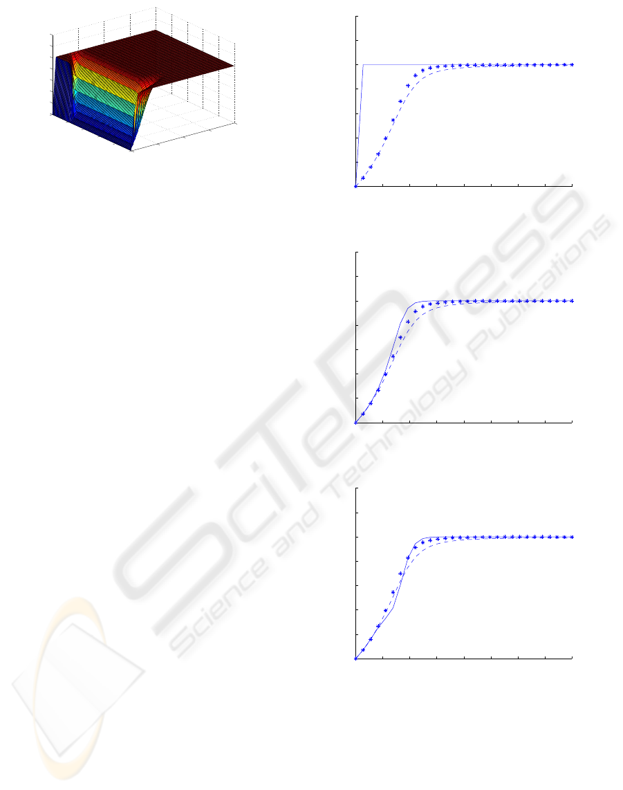
Figure 2 shows respectively the time evolution
of the concentration error e
2
at the positions 0.1 ∗ L,
0.5∗L and 0.9L, for the case where only the tempera-
ture is measured on the length interval [3∗L/4, L] (the
dashed line) i.e the exponential observer (18)-(21),
and for the case where both the temperature and the
concentration are measured on the same length inter-
val with the exponential observer (14)-(17) (the solid
line) and with the exponential observer (22)-(25) (the
star line).
It is seen as expected that the concentration error re-
lated to the exponential observer (22)-(25) is faster
than the one related to the exponential observer (18)-
(21), however it remains slower than that related to the
observer (14)-(17), which represents the ideal case,
since in that case, the nonlinear part is assumed to be
exactly known.
3 CONCLUSIONS
This paper presents sufficient conditions to construct
an exponential observer for a nonlinear infinite di-
mensional system driven in a real Hilbert state de-
scription. The theory is applied to a non-isothermal
plug flow tubular reactor governed by hyperbolic first
order partial differential equations. Several observer
structures are proposed, depending on the part of the
states that are available for measurement and on the
knowledge of the nonlinear part of the model. Per-
formance issues of the different observer designs are
illustrated by simulation results. The best perfor-
mance is obviously obtained when the nonlinear term
is perfectly known and both states (temperature and
concentration) are measured at the end of the reac-
tor. However, we also show that good results can be
achieved when only the temperature is measured and
when bounds on the nonlinear term are used in the ob-
0 0.1 0.2 0.3 0.4 0.5 0.6 0.7 0.8
−1
−0.8
−0.6
−0.4
−0.2
0
0.2
0.4
t
e2
(a) concentration error at z=0.9*L.
0 0.1 0.2 0.3 0.4 0.5 0.6 0.7 0.8
−1
−0.8
−0.6
−0.4
−0.2
0
0.2
0.4
t
e2
(b) concentration error at z=0.5*L.
0 0.1 0.2 0.3 0.4 0.5 0.6 0.7 0.8
−1
−0.8
−0.6
−0.4
−0.2
0
0.2
0.4
e2
(c) concentration error at z=0.1*L.
Figure 2: Convergence of the concentration error for the
three proposed observers.
server dynamics. Finally, an improved convergence
rate for the estimation error on the concentration can
be obtained when re-introducing a measurement of
the concentration at the end of the reactor. These ob-
servers include design parameters that can be tuned
by the user to satisfy specific needs in terms of con-
vergence rate.
ICINCO 2008 - International Conference on Informatics in Control, Automation and Robotics
26

REFERENCES
Achhab, M. E., Laabissi, M., Winkin, J., and Dochain, D.
(1999). State trajectory analysis of plug flow non-
isothermal reactors using a nonlinear model. In Pro-
ceedings of the 38th IEEE Conference on Decision
and Control, Phoenix, Arizona, USA, 663-667, De-
cember.
Aksikas, I., Winkin, J., and Dochain, D. (2007). Asymp-
totic stability of infinite-dimensional semilinear sys-
tems: application to a nonisothermal reactor. In Sys-
tems and Control Letters, vol. 56, 122-132.
Bounit, H. and Hammouri, H. (1997). Observers for infinite
dimensional bilinear systems. European J. of Control,
vol. 3, 325-339.
Cazenave, T. and Haraux, A. (1998). An Introduction to
Semilinear Evolution Equations. Clarendon Press.
Oxford.
Curtain, R. F. and Zwart, J. (1995). An Introduction to In-
finite Dimentional Linear Systems Theory. Springer,
New York.
Gauthier, J. P., Xu, C. Z., and Bounabat, A. (1995). Ob-
servers for infinite dimentional dissipative bilinear
systems. In J. Math. Systems, Estimation and Control,
vol. 5, 119-122.
Gressang, R. V. and Lamont, G. B. (1975). Observers for
systems characterized by semigroups. In IEEE Trans.
Aut. Contr, vol. 20, 523-528.
Laabissi, M., Achhab, M., Winkin, J., and Dochain, D.
(2001). Trajectory analysis of nonisothermal tubular
reactor nonlinear models. In Systems and Control Let-
ters, 42, 169-184.
Orlov, Y. and Dochain, D. (2002). Discontinuous feedback
stabilisation of minimum-phase semilinear infinite-
dimensional systems with application to chemical
tubular reactor models. In IEEE Trans. Aut. Contr,
vol. 47, 1293-1304.
Pazy, A. (1983). Semigroups of Linear Operators and Ap-
plications to Partial Differential Equations. Springer-
Verlag.
Smets, I., Dochain, D., and Impe, J. V. (2002). Optimal
temperature control of a steady-state exothermic plug-
flow reactor. In AIChE Journal, Vol. 48, No. 2, 279-
286.
Winkin, J., Dochain, D., and Ligarius, P. (2000). Dynamical
analysis of distributed parameter tubular reactors. In
Automatica, 36, 349-361.
EXPONENTIAL OBSERVER FOR A CLASS OF NONLINEAR DISTRIBUTED PARAMETER SYSTEMS WITH
APPLICATION TO A NONISOTHERMAL TUBULAR REACTOR
27