DYNAMICAL MODELS FOR OMNI-DIRECTIONAL ROBOTS WITH
3 AND 4 WHEELS
H
´
elder P. Oliveira, Armando J. Sousa, A. Paulo Moreira and Paulo J. Costa
Faculdade de Engenharia, Universidade do Porto, Rua Dr. Roberto Frias s/n 4200-465, Porto, Portugal
Keywords:
Identification, simulation, modeling and omni-directional mobile robots.
Abstract:
Omni-directional robots are becoming more and more common in recent robotic applications. They offer
improved ease of maneuverability and effectiveness at the expense of increased complexity. Frequent appli-
cations include but are not limited to robotic competitions and service robotics. The goal of this work is to
find a precise dynamical model in order to predict the robot behavior. Models were found for two real world
omni-directional robot configurations and their parameters estimated using a prototype that can have 3 or 4
wheels. Simulations and experimental runs are presented in order to validate the presented work.
1 INTRODUCTION
Omni-directional robots are becoming a much sought
solution to mobile robotic applications. This kind of
holonomic robots are interesting because they allow
greater maneuverability and efficiency at the expense
of some extra complexity. One of the most frequent
solutions is to use some of Mecanum wheels (Diegel
et al., 2002) and (Salih et al., 2006). A robot with 3
or more motorized wheels of this kind can have al-
most independent tangential, normal and angular ve-
locities. Dynamical models for this kind of robots are
not very common due to the difficulty in modeling
the several internal frictions inside the wheels, mak-
ing the model somewhat specific to the type of wheel
being used (Williams et al., 2002).
Frequent mechanical configurations for omni-
directional robots are based on three and four wheels.
Three wheeled systems are mechanically simpler but
robots with four wheels have more acceleration with
the same kind of motors. Four wheeled robots are
expected to have better effective floor traction, that
is, less wheel slippage – assuming that all wheels
are pressed against the floor equally. Of course four
wheeled robots also have a higher costs in equipment,
increased energy consumption and may require some
kind of suspension to distribute forces equally among
the wheels.
In order to study and compare the models of the
3 and 4 wheeled robots, a single prototype was built
that can have both configurations, that is, the same
mechanical platform can be used with 3 wheels and
then it can be disassembled and reassembled with a 4
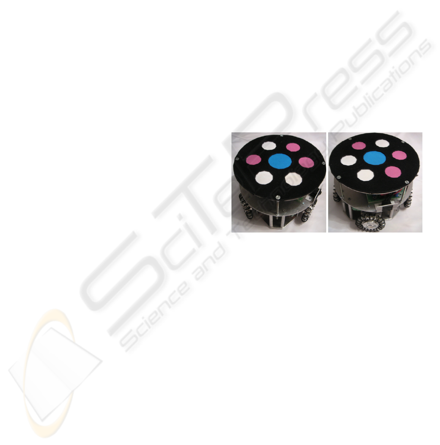
(a) Three wheeled robot. (b) Four wheeled robot.
Figure 1: Omni-directional robot.
wheel configuration, see figure 1.
Data from experimental runs is taken from over-
head camera. The setup is taken from the heritage
of the system described in (Costa et al., 2000) that
currently features 25 fps, one centimeter accuracy in
position(XX and YY axis) and about 3 sexagesimal
degrees of accuracy in the heading of the robot.
In order to increase the performance of robots,
there were some efforts on the studying their dy-
namical models (Campion et al., 1996)(Conceic¸
˜
ao
et al., 2006)(Khosla, 1989)(Tahmasebi et al.,
2005)(Williams et al., 2002) and kinematic models
(Campion et al., 1996) (Leow et al., 2002)(Loh et al.,
2003)(Muir and Neuman, 1987)(Xu et al., 2005).
Models are based on linear and non linear dynami-
cal systems and the estimation of parameters has been
the subject of continuing research (Conceic¸
˜
ao et al.,
2006)(Olsen and Petersen, 2001). Once the dynam-
ical model is found, its parameters have to be esti-
mated. The most common method for identification
189
P. Oliveira H., J. Sousa A., Paulo Moreira A. and J. Costa P. (2008).
DYNAMICAL MODELS FOR OMNI-DIRECTIONAL ROBOTS WITH 3 AND 4 WHEELS.
In Proceedings of the Fifth International Conference on Informatics in Control, Automation and Robotics - RA, pages 189-196
DOI: 10.5220/0001489201890196
Copyright
c
SciTePress
of robot parameters are based on the Least Squares
method and Instrumental Variables.
However, the systems are naturally non-linear
(Julier and Uhlmann, 1997), the estimation of pa-
rameters is more complex and the existing meth-
ods (Ghaharamani and Roweis, 1999)(Gordon et al.,
1993)(Tahmasebi et al., 2005) have to be adapted to
the model’s structure and noise.
1.1 Structure
This paper starts by presenting the mechanical proto-
type and studied mechanical configurations for the 3
and 4 wheeled robots. Finding the dynamical model is
discussed and then, an initial approach in estimating
model parameters for each robot is done. The need
for additional accuracy drives the comparative study
on relative importance of the estimated parameters.
An additional experiment is done for estimating fi-
nal numerical values for the configurations of 3 and
4 wheels. Conclusions and future work are also pre-
sented.
2 MECHANICAL
CONFIGURATIONS
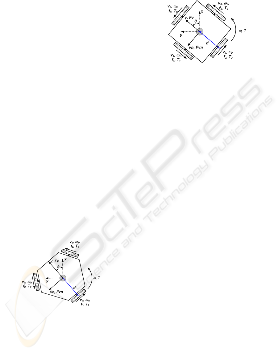
Figures 2 and 3 present the configuration of the three
and four wheeled robots respectively, as well as all
axis and relevant forces and velocities of the robotic
system. The three wheeled system features wheels
separated by 120 degrees.
Figure 2: Three Wheeled Robot.
Figures 2 and 3 show the notation used through-
out this paper, detailed as follows:
• x,y,θ - Robot’s position (x,y) and θ angle to the defined
front of robot;
• d [m] - Distance between wheels and center robot;
• v
0
,v
1
,v
2
,v
3
[m/s] - Wheels linear velocity;
• ω
0
,ω
1
,ω
2
,ω
3
[rad/s] - Wheels angular velocity;
• f
0
, f
1
, f
2
, f
3
[N] - Wheels traction force;
Figure 3: Four Wheeled Robot.
• T
0
,T
1
,T
2
,T
3
[N ·m] - Wheels traction torque;
• v, vn [m/s] - Robot linear velocity;
• ω [rad/s] - Robot angular velocity;
• F
v
,F
vn
[N] - Robot traction force along v and vn;
• T [N ·m] - Robot torque (respects to ω).
3 MODELS
3.1 Kinematic
The well known kinematic model of an omni-
directional robot located a (x,y, θ) can be written as
v
x
(t) = dx(t)/dt , v
y
(t) = dy(t)/dt and ω(t) = dθ(t)/dt
(please refer to figures 2 and 3 for notation issues).
Equation 1 allows the transformation from linear ve-
locities v
x
and v
y
on the static axis to linear velocities
v and vn on the robot’s axis.
X
R
=
v(t)
vn(t)
ω(t)
; X
0
=
v
x
(t)
v
y
(t)
ω(t)
X
R
=
cos(θ(t))
−sin(θ(t))
0
sin(θ(t))
cos(θ(t))
0
0
0
1
·X
0
(1)
3.1.1 Three Wheeled Robot
Wheel speeds v
0
, v
1
and v
2
are related with robot’s
speeds v, vn and ω as described by equation 2.
v
0
(t)
v
1
(t)
v
2
(t)
=
−sin(π/3)
0
sin(π/3)
cos(π/3)
−1
cos(π/3)
d
d
d
·
v(t)
vn(t)
ω(t)
(2)
Applying the inverse kinematics is possible to obtain
the equations that determine the robot speeds related
the wheels speed. Solving in order of v, vn and ω, the
following can be found:
v(t) = (
√
3/3) ·(v
2
(t)−v
0
(t)) (3)
vn(t) = (1/3)·(v
2
(t)+ v
0
(t))−(2/3)·v
1
(t) (4)
ω(t) = (1/(3 ·d))·(v
0
(t)+ v
1
(t)+ v
2
(t)) (5)
ICINCO 2008 - International Conference on Informatics in Control, Automation and Robotics
190

3.1.2 Four Wheeled Robot
The relationship between the wheels speed v
0
, v
1
, v
2
and v
3
, with the robot speeds v, vn and ω is described
by equation 6.
v
0
(t)
v
1
(t)
v
2
(t)
v
3
(t)
=
0
−1
0
1
1
0
−1
0
d
d
d
d
·
v(t)
vn(t)
ω(t)
(6)
It is possible to obtain the equations that determine the
robot speeds related with wheels speed but the matrix
associated with equation 6 is not square. This is be-
cause the system is redundant. It can be found that:
v(t) = (1/2)·(v
3
(t)−v
1
(t)) (7)
vn(t) = (1/2)·(v
0
(t)−v
2
(t)) (8)
ω(t) = (v
0
(t)+ v
1
(t)+ v
2
(t)+ v
3
(t))/(4 ·d) (9)
3.2 Dynamic
The dynamical equations relative to the accelerations
can be described in the following relations:
M ·
dv(t)
dt
=
∑
F
v
(t)−F
Bv
(t)−F
Cv
(t) (10)
M ·
dvn(t)
dt
=
∑
F
vn
(t)−F
Bvn
(t)−F
Cvn
(t) (11)
J ·
dω(t)
dt
=
∑
T (t) −T
Bω
(t)−T
Cω
(t) (12)
where the following parameters relate to the robot as
follows:
• M [kg] - mass;
• J [kg ·m
2
] - inertia moment;
• F
Bv
,F
Bvn
[N] - viscous friction forces along v and vn;
• T
Bω
[N ·m] - viscous friction torque with respect to the
robot’s rotation axis;
• F
Cv
,F
Cvn
[N] - Coulomb frictions forces along v and vn;
• T
Cω
[N ·m] - Coulomb friction torque with respect to
robot’s rotation axis.
Viscous friction forces are proportional to robot’s
speed and as such F
Bv
(t) = B
v
·v(t), F
Bvn
(t) = B
vn
·vn(t)
and T
Bω
(t) = B
ω
·ω(t), where Bv,Bvn [N/(m/s)] are the
viscous friction coefficients for directions v and vn
and Bω [N ·m/(rad/s)] is the viscous friction coeffi-
cient to ω.
The Coulomb friction forces are constant in am-
plitude F
Cv
(t) = C
v
·sign(v(t)), F
Cvn
(t) = C
vn
·sign(vn(t))
and T
Cω
(t) = C
ω
· sign ω(t), where Cv,Cvn [N] are
Coulomb friction coefficient for directions v e vn and
Cω [N ·m] is the Coulomb friction coefficient for ω.
3.2.1 Three Wheeled Robot
The relationship between the traction forces and rota-
tion torque of the robot with the traction forces on the
wheels is described by the following equations:
∑
F
v
(t) = ( f
2
(t)− f
0
(t))·sin(π/3) (13)
∑
F
vn
(t) = −f
1
(t)+ ( f
2
(t)+ f
0
(t))·cos(π/3)(14)
∑
T (t) = ( f
0
(t)+ f
1
(t)+ f
2
(t))·d (15)
The traction force on each wheel is estimated by trac-
tion torque, which can be determined using the motor
current, as described in the following equations:
f
j
(t) = T
j
(t)/r (16)
T
j
(t) = l ·K
t
·i
j
(t) (17)
• l - Gearbox reduction;
• r [m] - Wheel radius;
• K
t
[N ·m/A] - Motor torque constant;
• i
j
[A] - Motor current (j=motor number).
3.2.2 Four Wheeled Robot
The relationship between the traction forces and rota-
tion torque of the robot with the traction forces on the
wheels, is described by the following equations:
∑
F
v
(t) = f
3
(t)− f
1
(t) (18)
∑
F
vn
(t) = f
0
(t)− f
2
(t) (19)
∑
T (t) = ( f
0
(t)+ f
1
(t)+ f
2
(t)+ f
3
(t))·d (20)
As above, the traction force in each wheel is esti-
mated using the wheels traction torque, which is de-
termined by the motor current, using equations 16 and
17, where j=0,1,2,3.
3.3 Motor
The prototype uses brushless motors for the locomo-
tion of the robot. The model for brushless motors is
the similar to the common DC motors, based on (Pil-
lay and Krishnan, 1989).
u
j
(t) = L ·
di
j
(t)
dt
+ R ·i
j
(t)+ K
v
·ω
m j
(t) (21)
T
m j
(t) = K
t
·i
j
(t) (22)
• L [H] - Motor inductance;
• R [Ω] - Motor resistor;
• K
v
[V /(rad/s)] - EMF motor constant;
• u
j
[V ] - Motor voltage (j=motor number);
• ω
m j
[rad/s] - Motor angular velocity (j=motor num-
ber);
• T
m j
[N ·m] - Motor torque (j=motor number).
DYNAMICAL MODELS FOR OMNI-DIRECTIONAL ROBOTS WITH 3 AND 4 WHEELS
191

4 PARAMETER ESTIMATION
The necessary variables to estimate the model param-
eters are motor current, robot position and velocity.
Currents are measured by the drive electronics, posi-
tion is measured by using external camera and veloc-
ities are estimated from positions.
The parameters that must be identified are the vis-
cous friction coefficients (Bv,Bvn, Bω), the Coulomb
friction coefficients (Cv,Cvn,Cω) and inertia moment
J. The robot mass was measured, and it was 1.944 k g
for the three wheeled robot and 2.34 kg for the four
wheeled robot.
4.1 Experience 1 - Steady State Velocity
This method permits to identify the viscous friction
coefficients Bω and the Coulomb friction coefficients
Cω. The estimation of the coefficient ω was only im-
plemented because inertia moment is unknown, and it
is necessary to have an initial estimate of these coef-
ficients. The experimental method relies on applying
different voltages to the motors in order to move the
robot according his rotation axis - the tests were made
for positive velocities. Once reached the steady state,
the robot’s speed ω and rotation torque T can be mea-
sured. The robot speed is constant, so, the accelera-
tion is null, and as such equation 12 can be re-written
as follows:
∑
T (t) = B
ω
·ω(t) +C
ω
(23)
This linear equation shows that it is possible to test
different values of rotation speed and rotation torques
in multiple experiences and estimate the parameters.
4.2 Experience 2 - Null Traction Forces
This method allows for the estimation of the viscous
friction coefficients (Bv, Bvn), the Coulomb friction
coefficients (Cv,Cvn) and the inertia moment J. The
experimental method consists in measuring the robot
acceleration and speed when the traction forces were
null. The motor connectors were disconnected and
with a manual movement starting from a stable posi-
tion, the robot was pushed through the directions v,
vn and rotated according to his rotation axis. During
the subsequent deceleration, velocity and acceleration
were measured. Because the traction forces were null
during the deceleration equations 10, 11, and 12 can
be re-written as follows:
dv(t)
dt
= −
B
v
M
·v(t) −
C
v
M
(24)
dvn(t)
dt
= −
B
vn
M
·vn(t) −
C
vn
M
(25)
dω(t)
dt
= −
B
ω
J
·ω(t) −
C
ω
J
(26)
These equations are also a linear relation and estima-
tion of all parameters is possible.
The inertia moment J is estimated using the values
obtained previously in section 4.1. To do this, equa-
tion 26 must be solved in order of J:
J = −
ω(t)
(dω(t)/dt)
·B
ω
−
1
(dω(t)/dt)
·C
ω
(27)
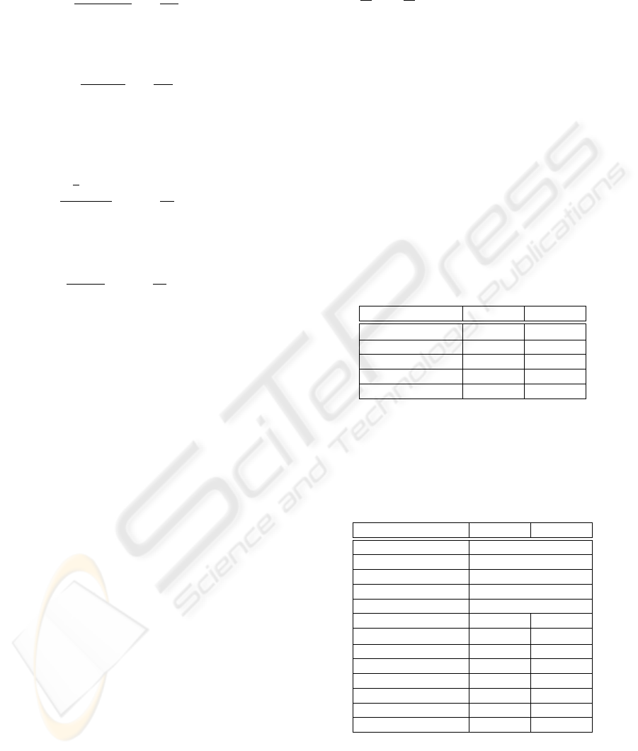
4.3 DC Motor Parameters
The previous electrical motor model (equation 21) in-
cludes an electrical pole and a much slower, dominant
mechanical pole - thus making inductance L value
negligible. To determinate the relevant parameters K
v
and R, a constant voltage is applied to the motor. Un-
der steady state condition, the motor’s current and the
robot’s angular velocity are measured. The tests are
repeated several times for the same voltage, chang-
ing the operation point of the motor, by changing the
friction on the motor axis.
In steady state, the inductance L disappears of the
equation 21, being rewritten as follows:
u
j
(t) = R ·i
j
(t)+ K
v
·ω
m j
(t) (28)
As seen in equation 29, by dividing (28) by i
j
(t), a
linear relation is obtained and thus estimation is pos-
sible.
u
j
(t)
i
j
(t)
= K
v
·
ω
m j
(t)
i
j
(t)
+ R (29)
5 RESULTS
5.1 Robot Model
By combining previously mentioned equations, it is
possible to show that model equations can be rear-
ranged into a variation of the state space that can be
described as:
(dx(t)/dt) = A ·x(t) +B ·u(t) + K ·sign(x) (30)
x(t) = [v(t) vn(t) w(t)]
T
(31)
This formulation is interesting because it shows ex-
actly which part of the system is non non-linear.
5.1.1 Three Wheeled
Using equations on section 3.2, 13 to 17 and 28, the
equations for the three wheeled robot model are:
A =
A
11
0
0
0
A
22
0
0
0
A
33
(32)
A
11
= −
3 ·K
2
t
·l
2
2 ·r
2
·R ·M
−
B
v
M
A
22
= −
3 ·K
2
t
·l
2
2 ·r
2
·R ·M
−
B
vn
M
A
33
= −
3 ·d
2
·K
2
t
·l
2
r
2
·R ·J
−
B
w
J
ICINCO 2008 - International Conference on Informatics in Control, Automation and Robotics
192
B =
l ·K
t
r ·R
·
−
√
3/(2 ·M)
1/(2 ·M)
d/J
0
1/M
d/J
√
3/(2 ·M)
1/(2 ·M)
d/J
(33)
K =
−C
v
/M
0
0
0
−C
vn
/M
0
0
0
−C
w
/J
(34)
5.1.2 Four Wheeled
Using equations on section 3.2 and equations 16 to
20 and 28 we get the following equations to the four
wheeled robot model.
A =
A
11
0
0
0
A
22
0
0
0
A
33
(35)
A
11
= −
2 ·K
2
t
·l
2
r
2
·R ·M
−
B
v
M
A
22
= −
2 ·K
2
t
·l
2
r
2
·R ·M
−
B
vn
M
A
33
= −
4 ·d
2
·K
2
t
·l
2
r
2
·R ·J
−
B
w
J
B =
l ·K
t
r ·R
·
0
1/M
d/J
−1/M
0
d/J
0
−1/M
d/J
1/M
0
d/J
(36)
K =
−C
v
/M
0
0
0
−C
vn
/M
0
0
0
−C
w
/J
(37)
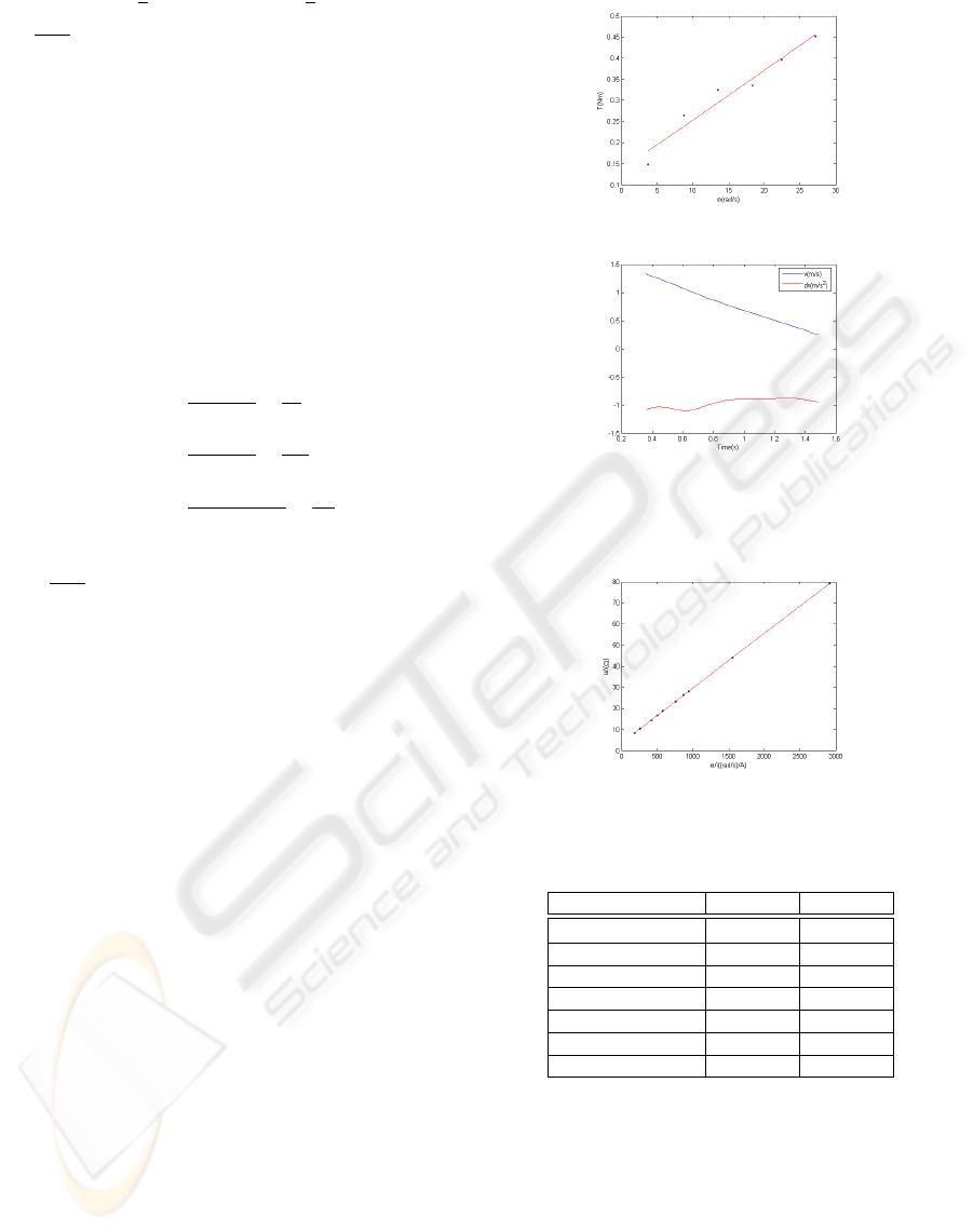
5.2 Experimental Data for Robot Model
Experience 1 was conducted using an input signal cor-
responding to a ramped up step. This way wheel
sleeping was avoided, that is, wheel - traction prob-
lems don’t exist.
Shown in Figure 4 are the experimental plots re-
garding the 4 wheeled system. Due to space con-
straints only T vs. ω and results of the experiment 2
along the v direction are shown.
The motor model was presented earlier in equa-
tion 21.
Experimental tests to the four motors were made
to estimate the value of resistor R and the constant
K
v
. The numerical value of the torque constant K
t
is
identical to the EMF motor constant K
v
.
Figure 5 plots experimental runs regarding motor
0. Other motors follow similar behavior.
5.3 Numerical Results
Table 1 presents the experimental results to the fric-
tion coefficients and inertial moment. From the exper-
imental runs from all 4 motors, the parameters found
are K
v
= 0.0259 V /(rad/s) and R = 3.7007 Ω .
(a) Experience 1 - T and ω.
(b) Experience 2 - Direction v.
Figure 4: Experimental Results for the four wheeled robot.
Figure 5: Experimental tests for motor 0.
Table 1: Friction coefficients and inertia moment.
Parameters 3 wheels 4 wheels
J(kg ·m
2
) 0.015 0.016
B
v
(N/(m/s)) 0.503 0.477
B
vn
(N/(m/s)) 0.516 0.600
B
ω
N ·m/(rad/s) 0.011 0.011
C
v
(N) 1.906 1.873
C
vn
(N) 2.042 2.219
C
ω
(N ·m) 0.113 0.135
5.4 Sensitivity Analysis
To understand which model parameters have more in-
fluence on the robot’s dynamics, a comparison was
made between the matrices of the models.
The model equation 30 is a sum of fractions. Ana-
lyzing the contribution of each parcel and of the vari-
able portion within each fraction, a sensitivity analy-
sis is performed, one estimated parameter at a time.
DYNAMICAL MODELS FOR OMNI-DIRECTIONAL ROBOTS WITH 3 AND 4 WHEELS
193
1. Matrix A, robot moving along v direction;
• Three wheeled robot:
3 ·K
2
t
·l
2
2 ·r
2
·R ·M
=
K
a1
R
= 3.3110
(B
v
/M) = K
a2
·B
v
= 0.3245
• Four wheeled robot:
2 ·K
2
t
·l
2
r
2
·R ·M
=
K
a1
R
= 3.6676
(B
v
/M) = K
a2
·B
v
= 0.2041
2. Matrices B and K, robot moving along v direction with
constant voltage motor equal to 6V ;
• Three wheeled robot:
√
3 ·l ·K
t
2 ·r ·R ·M
!
·12 =
K
b
R
·12 = 5.7570
(C
v
/M) = K
k
·C
v
= 0.8728
• Four wheeled robot:
l ·K
t
r ·R ·M
·12 =
K
b
R
·12 = 5.5227
(C
v
/M) = K
k
·C
v
= 0.7879
The same kind of analysis could be taken further by
analyzing other velocities (vn and ω). Conclusions
reaffirm that motor parameters have more influence
in the dynamics than friction coefficients. This means
that it is very important to have an accurate estima-
tion of the motor parameters. Some additional ex-
periences were designed to improve accuracy. The
method used previously does not offer sufficient ac-
curacy to the estimation of R. This parameter R is
not a physical parameter and includes a portion of the
non-linearity of the H bridge powering the circuit that,
in turn, feeds 3 rapidly switching phases of the brush-
less motors used. In conclusion, additional accuracy
in estimating R is needed.
5.5 Experience 3 - Parameter
Estimation Improvement
The parameter improving experience was made using
a step voltage with an initial acceleration ramp.
As seen in 5.1 the model was defined by the equa-
tion 30 and we can improve the quality of the estima-
tion by using the Least Squares method. The system
model equation can be rewritten as:
y = θ
1
·x
1
+ θ
2
·x
2
+ θ
3
·x
3
(38)
Where x
1
= x(t), x
2
= u(t), x
3
= 1 and y = dx(t)/dt. The
parameters θ are estimated using:
θ =
x
T
·x
−1
·x
T
·y (39)
x = [x
1
(1)...x
1
(n) x
2
(1)...x
2
(n) x
3
(1)...x
3
(n)]
T
(40)
Estimated parameters can be skewed and for this rea-
son instrumental variables are used to minimize the
error, with vector of states defined as
z = [x
1
(1)...x
1
(n) x
2
(1)...x
2
(n) x
3
(1)...x
3
(n)]
T
(41)
The parameters θ are now calculated by:
θ =
z
T
·x
−1
·z
T
·y (42)
Three experiments were made for each configuration
of 3 and 4 wheels, along v, vn and ω. For the v and
vn experiments values C
v
and C
vn
are kept from pre-
vious analysis. For the ω experiment, the value of
the R parameter used is the already improved version
from previous v and vn experimental runs of the cur-
rent section.
The numerical value of R for each motor was
estimated for each motor and then averaged to find
R=4.3111 Ω. The results are present on followings ta-
bles. Table 2 shows values estimated by the experi-
ment mentioned in this section.
Table 2: Parameters estimated using the method 3.
Parameters 3 wheels 4 wheels
J(kg ·m
2
) 0.0187 0.0288
B
v
(N/(m/s)) 0.5134 0.5181
B
vn
(N/(m/s)) 0.4571 0.7518
B
ω
N ·m/(rad/s) 0.0150 0.0165
C
ω
(N ·m) 0.0812 0.1411
The final values for friction and inertial coeffi-
cients are averaged with results from all 3 experimen-
tal methods and the numerical values found are pre-
sented in Table 3.
Table 3: Parameters of dynamical models.
Parameters 3 wheels 4 wheels
d(m) 0.089
r (m) 0.0325
l 5
K
v
(V /(rad/s)) 0.0259
R (Ω) 4.3111
M(kg) 1.944 2.34
J (kg ·m
2
) 0.0169 0.0228
B
v
(N/(m/s)) 0.5082 0.4978
B
vn
(N/(m/s)) 0.4870 0.6763
B
ω
(N ·m/(rad/s)) 0.0130 0.0141
C
v
(N) 1.9068 1.8738
C
vn
(N) 2.0423 2.2198
C
ω
(N ·m) 0.0971 0.1385
5.6 Model Validation Experiences
The models were validated with experimental tests on
using a step voltage with an initial acceleration ramp.
ICINCO 2008 - International Conference on Informatics in Control, Automation and Robotics
194
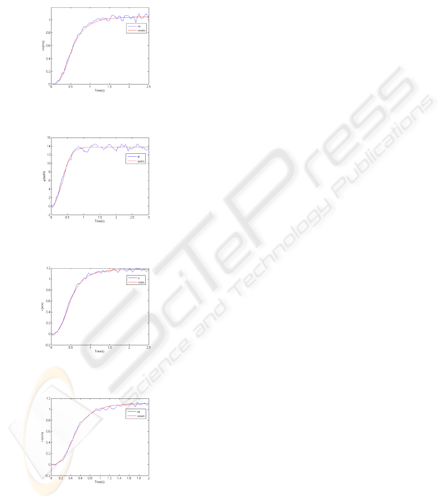
Due to space constraints in this document, figures 6
to 9 show plots for some of the runs only. Other runs
confirm the global validity of the model as simulation
follows reality closely.
Figure 6: 3 wheel model validation - velocity along vn.
Figure 7: 3 wheel model validation - angular velocity ω.
Figure 8: 4 wheel model validation - velocity along v.
Figure 9: 4 wheel model validation - velocity along vn.
6 CONCLUSIONS
This paper presents models for mobile omni-
directional robots with 3 and 4 wheels. The derived
model is non-linear but maintains some similarities
with linear state space equations. Friction coefficients
are most likely dependent on robot and wheels con-
struction and also on the weight of the robot. The
model is derived assuming no wheel slip as in most
standard robotic applications.
A prototype that can have either 3 or 4 omni-
directional wheels was used to validate the presented
model. The test ground is smooth and carpeted. Expe-
rience data was gathered by overhead camera capable
of determining position and orientation of the robot
with good accuracy.
Experiences were made to estimate the parame-
ters of the model for the prototypes. The accuracy of
the presented model is discussed and the need for ad-
ditional experiences is proved. The initial estimation
method used two experiences to find all parameters
but a third experience is needed to improve the accu-
racy of the most important model parameters. Sen-
sitivity analysis shows that the most important model
parameters concern motor constants.
Observing estimated model parameters, the four
wheel robot has higher friction coefficients in the vn
direction when compared to the v direction. This
means of course higher maximum speed for move-
ment along v axis and higher power consumption for
movements along the vn direction. This difference in
performance points to the need of mechanical suspen-
sion to even wheel pressure on the ground.
The found model was shown to be adequate for the
prototypes in the several shown experimental runs.
7 FUTURE WORK
The work presented is part of a larger study. Fu-
ture work will include further tests with different pro-
totypes including prototypes with suspension. The
model can also be enlarged to include the limits for
slippage and movement with controlled slip for the
purpose of studying traction problems. Dynamical
models estimated in this work can be used to study the
limitations of the mechanical configuration and allow
for future enhancements both at controller and me-
chanical configuration level. This study will enable
effective full comparison of 3 and 4 wheeled systems.
DYNAMICAL MODELS FOR OMNI-DIRECTIONAL ROBOTS WITH 3 AND 4 WHEELS
195

REFERENCES
Campion, G., Bastin, G., and Dandrea-Novel, B. (1996).
Structural properties and classification of kinematic
and dynamic models of wheeled mobile robots. IEEE
Transactions on Robotics and Automation, 12(1):47–
62. 1042-296X.
Conceic¸
˜
ao, A. S., Moreira, A. P., and Costa, P. J.
(2006). Model identification of a four wheeled omni-
directional mobile robot. In Controlo 2006, 7th Por-
tuguese Conference on Automatic Control, Instituto
Superior T
´
ecnico, Lisboa, Portugal.
Costa, P., Marques, P., Moreira, A. P., Sousa, A., and Costa,
P. (2000). Tracking and identifying in real time the
robots of a f-180 team. In Manuela Veloso, Enrico
Pagello and Hiroaki Kitano, Robocup-99: Robot Soc-
cer World Cup III. Springer, LNAI, pages 289–291.
Diegel, O., Badve, A., Bright, G., Potgieter, and Tlale, S.
(2002). Improved mecanum wheel design for omni-
directional robots. In Proc. 2002 Australasian Con-
ference on Robotics and Automation, Auckland.
Ghaharamani, Z. and Roweis, S. T. (1999). Learning non-
linear dynamical systems using an em algorithm. In
M. S. Kearns, S. A. Solla, D. A. Cohn, (eds) Ad-
vances in Neural Information Processing Systems.
Cambridge, MA: MIT Press, 11.
Gordon, N. J., Salmond, D. J., and Smith, A. F. M. (1993).
Novel approach to nonlinear/non-gaussian bayesian
state estimation. IEE Proceedings-F on Radar and
Signal Processing,, 140(2):107–113. 0956-375X.
Julier, S. J. and Uhlmann, J. K. (1997). A new extension
of the kalman filter to nonlinear systems. Int. Symp.
Aerospace/Defense Sensing, Simul. and Controls, Or-
lando, FL.
Khosla, P. K. (1989). Categorization of parameters in the
dynamic robot model. IEEE Transactions on Robotics
and Automation, 5(3):261–268. 1042-296X.
Leow, Y. P., H., L. K., and K., L. W. (2002). Kinematic
modelling and analysis of mobile robots with omni-
directional wheels. In Seventh lnternational Confer-
ence on Control, Automation, Robotics And Vision
(lCARCV’O2), Singapore.
Loh, W. K., Low, K. H., and Leow, Y. P. (2003). Mecha-
tronics design and kinematic modelling of a singu-
larityless omni-directional wheeled mobile robot. In
Robotics and Automation, 2003. Proceedings. ICRA
’03. IEEE International Conference on, volume 3,
pages 3237–3242.
Muir, P. and Neuman, C. (1987). Kinematic modeling for
feedback control of an omnidirectional wheeled mo-
bile robot. In Proceedings 1987 IEEE International
Conference on Robotics and Automation, volume 4,
pages 1772–1778.
Olsen, M. M. and Petersen, H. G. (2001). A new
method for estimating parameters of a dynamic robot
model. IEEE Transactions on Robotics and Automa-
tion, 17(1):95–100. 1042-296X.
Pillay, P. and Krishnan, R. (1989). Modeling, simulation,
and analysis of permanent-magnet motor drives, part
11: The brushless dc motor drive. IEEE transactions
on Industry applications, 25(2):274–279.
Salih, J., Rizon, M., Yaacob, S., Adom, A., and Mamat,
M. (2006). Designing omni-directional mobile robot
with mecanum wheel. American Journal of Applied
Sciences, 3(5):1831–1835.
Tahmasebi, A. M., Taati, B., Mobasser, F., and Hashtrudi-
Zaad, K. (2005). Dynamic parameter identification
and analysis of a phantom haptic device. In Proceed-
ings of 2005 IEEE Conference on Control Applica-
tions, pages 1251–1256.
Williams, R. L., I., Carter, B. E., Gallina, P., and Rosati, G.
(2002). Dynamic model with slip for wheeled omnidi-
rectional robots. IEEE Transactions on Robotics and
Automation, 18(3):285–293. 1042-296X.
Xu, J., Zhang, M., and Zhang, J. (2005). Kinematic model
identification of autonomous mobile robot using dy-
namical recurrent neural networks. In 2005 IEEE
International Conference Mechatronics and Automa-
tion, volume 3, pages 1447–1450.
ICINCO 2008 - International Conference on Informatics in Control, Automation and Robotics
196
