COLLISION AVOIDANCE SYSTEM PRORETA
Strategies Trajectory Control and Test Drives
R. Isermann, U. Stählin and M. Schorn
Institute of Automatic Control, Technische Universität Darmstadt
Landgraf-Georg-Str. 4, 64283 Darmstadt, Germany
Keywords: Collision avoidance, vehicle, object detection, path following, automatic braking, automatic steering.
Abstract: Methods and experimental results of a collision avoidance driver assistance system are described with
automatic object detection, trajectory prediction, and path following with controlled braking and steering.
The objects are detected by a fusion of LIDAR scanning and video camera pictures resulting in the location,
size and speed of objects in front of the car. A desired trajectory is calculated depending on the distance, the
width of a swerving action and difference speed. For the trajectory control different control methods were
designed and tested experimentally like velocity depend linear feedback and feedforward control, nonlinear
asymptotic output tracking and nonlinear flatness based control using extended one-track models with
vehicle state estimation for the sideslip angle and cornering stiffness. Automatic braking is realized with an
electrohydraulic brake (EHB) and automatic steering with an active front steering (AFS). The various
control systems are compared by simulations and real test drives showing the behaviour of a VW Golf with
automatic braking or/and automatic swerving to a free track, such avoiding hitting a suddenly appearing
obstacle. The research project PRORETA was a four-years-cooperation between Continental Automotive
Systems and Darmstadt University of Technology.
1 INTRODUCTION
Driver Assistance Systems for Collision Avoidance
have the goal to prevent accidents using braking or
evasive maneuvers. An automatic collision
avoidance system has to monitor its surroundings,
detect an upcoming accident and intervene
appropriately to avoid the accident. In case of the
system developed by the research project
PRORETA – Electronic Driver Assistance System
for a Collision Avoiding Vehicle, a cooperation
between Technische Universität Darmstadt and
Continental AG, the driver is given the chance to
avoid the accident himself as long as possible.
Therefore, the interventions have to be conducted at
the physical last possible moment or the driving
dynamics stability boundary.
Using these predictions, a decision is made,
whether an intervention is necessary or not and the
intervention is planned. The intervention itself is
then conducted fully automatically. An ergonomic
study accompanied the development of the system.
This study investigated how the driver reacts in
critical situations and how he reacts on the
interventions by PRORETA.
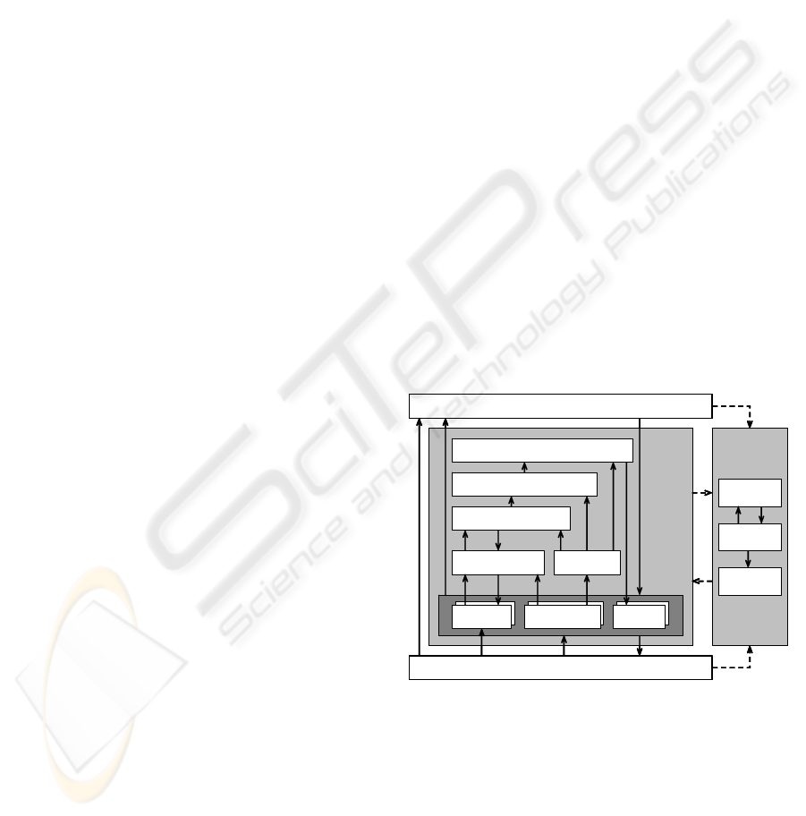
Environment
Driver
Control
Sensors for
vehicle states
Vehicle state
estimation
Intervention planning
Environmental
sensors
Fusion of environmental
sensors and state estimation
for the environment
Trajectory prediction
PRORETA
prototype
Vehicle
Actuators
Experiments
with test persons
Analysis
Ergonomic
studies
Reactions of drivers,
design notes,
acceptance
Figure 1: System overview prorate.
In this contribution, the intervention decision, the
planning of the intervention and the conduction of
the intervention are described. The environment
perception is described in detail in (Darms and
Winner, 2006). Results from the ergonomic study
can be found in (Bender and Landau, K., 2006). The
system was tested using a complex two track model
followed by extensive driving tests with an
experimental vehicle.
35
Isermann R., Stählin U. and Schorn M. (2008).
COLLISION AVOIDANCE SYSTEM PRORETA - Strategies Trajectory Control and Test Drives.
In Proceedings of the Fifth Inter national Conference on Informatics in Control, Automation and Robotics - ICSO, pages 35-42
DOI: 10.5220/0001489300350042
Copyright
c
SciTePress
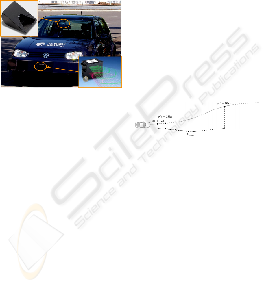
2 TEST VEHICLE
A VW Golf IV, which was only equipped with
additional sensors and actuators required for the
developed functions, served as experimental vehicle,
see Figure 2.
Figure 2: Environmental Sensors of the test vehicle.
The driver assistance system uses an active front
steering and an electro hydraulic braking system as
actuators. For vehicle state estimation only ESP
sensors and the sensors of the active front steering
and braking system are necessary. For environment
perception a laser scanner and a video sensor were
used. The chosen design allows to scan the area in
front of the vehicle. The detection area of the laser
scanner covers an angular range of 22.5° with a
resolution of 1.5° and is scanned in a 90 ms cycle.
The distance to objects is determined by a time of
flight measurement of emitted light impulses. The
video sensor is based on a monochrome CMOS
image sensor that provides data in a 40 ms cycle.
The detection area is 44°, whereas the discretisation
with approx. 0.07° is considerably finer than for the
laser scanner. By means of image processing
algorithms, vehicle rear views and lane markings
can be detected in the image, however, a direct
distance measurement is not possible, for details see
(Darms and Winner, 2006).
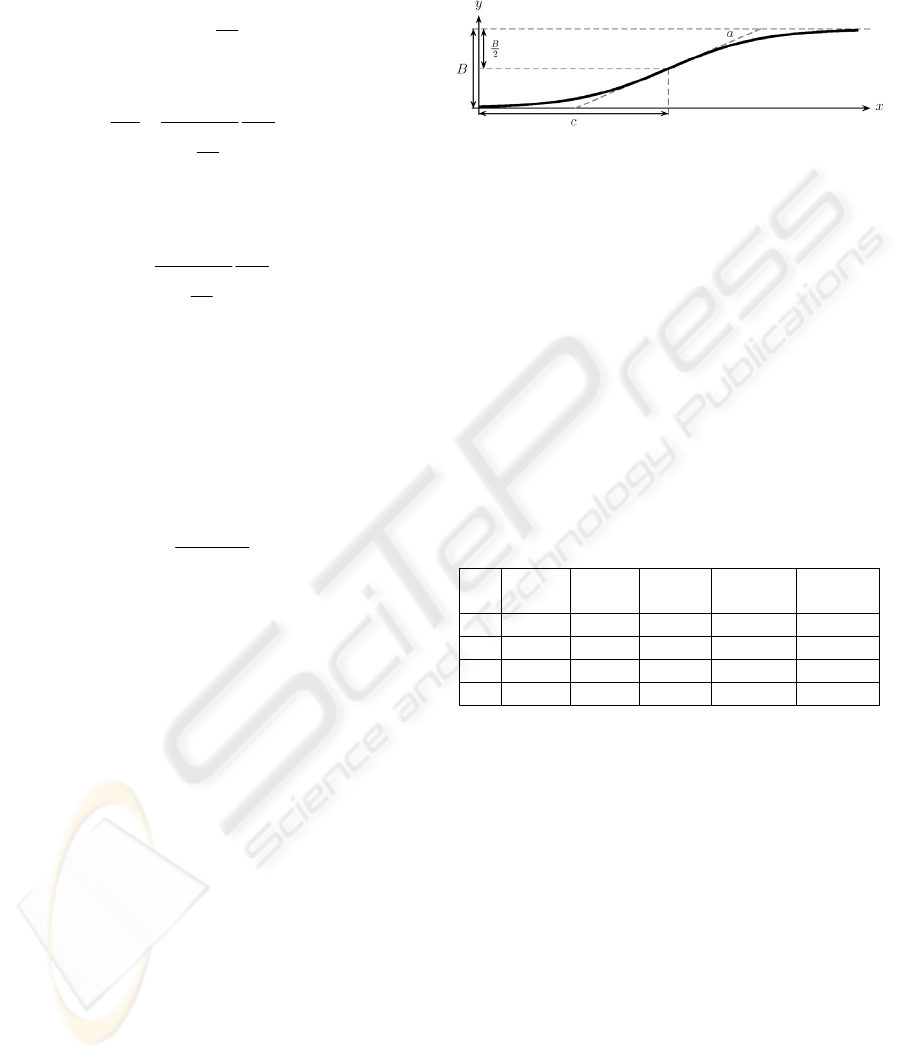
3 EVASIVE TRAJECTORY
An evasive trajectory is required between
intervention planning and control For investigating
several different intervention functions with
different types of controllers, the type of
intervention is selected using some flags. The flags
used in this article are braking, emergency braking
and evasion. If braking is chosen, the desired
deceleration has to be transmitted. If an emergency
braking is chosen, the maximum possible
deceleration at every point in time is achieved using
braking controllers. For an evasion, the desired
position and heading are given for one time step T
B
,
two time steps T
B
and ten time steps T
B
ahead in
time, Figure 3. The coordinate system used is
stationary for the duration of the evasion and is
initialized at the beginning of the evasion to match
the vehicle coordinate system at that point. The last
position, which is supposed to be reached 10 time
steps in the future, is used to make sure the
controller can react predictively on deviations of the
first 2 time steps. Figure 3 shows this interface.
Every point p(t) consists of the position (x, y) and
the heading
ψ
of the vehicle. All three points are put
together in one matrix transmitted to the controller:
(
)
(
)
(
)
210
evasion
pt T pt T pt T
B
BB
⎡
⎤
=+ + +
⎢
⎥
⎣
⎦
P
Figure 3: Evasive trajectory between planning and control.
4 PLANNING OF THE EVASIVE
INTERVENTION
Primary goal of the evasive trajectory is to reach a
predefined lateral offset with the shortest possible
traveled path. The designed trajectory has to be
feasible regarding the vehicle dynamics laws and
after the maneuver the vehicle has to be in a safe and
stable state.
Vehicle dynamics laws of the trajectory are
taken into account to limit the maximum allowed
lateral acceleration. This limit can be adapted to the
actual traffic and driving situation, especially
weather conditions. The steering actuator also limits
the maximum possible jerk.
Since the trajectory is transmitted to the
controller using positions, the general relations
between the position on the trajectory and the
driving dynamics are considered first. This relation
is based on the simple equations of the one-track
model and the Ackermann equations. The approach
shown here uses a relation where the y-position on
the trajectory is depended on the x-position:
ICINCO 2008 - International Conference on Informatics in Control, Automation and Robotics
36
()yfx=
(1)
Using geometric transformations, the yaw angle
ψ
can be expressed as (assuming no side slip)
arctan
dy
dx
ψ
⎛⎞
=
⎜⎟
⎝⎠
(2)
and therefore its derivative regarding time yields:
2
2
2
1
1
x
ddy
v
dt dx
dy
dx
ψ
ψ
==
⎛⎞
+
⎜⎟
⎝⎠
&
(3)
Based on this and using the Ackermann relations,
the lateral acceleration is:
2
2
2
1
1
yx
dy
av vv
dx
dy
dx
ψ
==
⎛⎞
+
⎜⎟
⎝⎠
&
(4)
Further simplification can be accomplished
assuming
vv
x
= .
Often, a sequence of klothoids is used for the
evasive trajectory, see e.g. (Ameling, 2002). In
general, trajectories for evasive maneuvers have the
shape of a lying S. Functions describing such a
shape are called sigmoidal functions or sigmoides.
In the following a sigmoide of the form
()
()
1
ax c
B
yx
e
−−
=
+
(5)
is used. B is the maneuver width, describing the
distance between minimum and maximum y-value. a
defines the slope of the sigmoide, where high values
for a are leading to a steeper curve. c defines the
position of the inflection point and therefore the
length of the evasive maneuver, which is s=2c.
Looking at equation (5), the sigmoide has its
maximum and minimum at infinity, meaning
lim ( ) 0
x
yx
→−∞
=
(6)
and
lim ( )
x
yx B
→∞
=
(7)
respectively. Therefore, an additional parameter
Tol
y is introduced. Using this parameter, the
following counts:
Tol
(0)yy=
(8)
and
Tol
(2 )yc By=−
(9)
Figure 4 shows this sigmoide and the respective
parameters. The parameters can be chosen according
to the driving situation, such that the evasive path is
minimal regarding the limitations for maximum
lateral acceleration, maximal jerk and dynamics of
the steering actuator. The derivation of the
respective parameters can be found in (Stählin et al.,
2006).
Figure 4: Evasive sigmoide and its parameters.
The most important value for taking a decision,
whether the klothoide or the sigmoide should be
chosen for the evasive trajectory is the length s of
the path of the evasive maneuver, taking into
account the limiting factors (maximum lateral
acceleration, maximum jerk,…). Table 1 shows a
comparison between klothoide and sigmoide for
different limiting factors. It can be seen, that the
sigmoide always leads to a shorter path for the
evasive maneuver. This is due to the linear increase
of the lateral acceleration for the klothoide in
comparison to the faster and nonlinear increase in
lateral acceleration for the sigmoide. Both
trajectories can be realized by a controller trajectory.
Table 1: Comparison of the length of an evasion for
klothoide and sigmoide with y
A
=y
m.
B v lateral
accel.
jerk Klothoide Sigmoide
2m 15m/s 5m/s2 30m/s3 26,83m 22,08m
3m 15m/s 5m/s2 30m/s3 32,85m 29,10m
2m 36m/s 5m/s2 30m/s3 64,30m 53,39m
3m 36m/s 5m/s2 30m/s3 78,85m 70,42m
5 INTERVENTION DECISION
Based on the fused environment data it is decided if
a collision is likely to occur and if so, which
maneuver has to be carried out to avoid the collision.
The strategy is to avoid the collision at the
physically last possible moment by an intervention
in order to give the driver the possibility to defuse
the critical situation by his own actions as long as
possible.
In order to determine a threatening collision,
predictions are first made for the own vehicle
driving tube and the movement of the objects in the
environment. By means of these predictions it can
then be predicted whether a collision will occur. If
this is the case, it is planned in a next step when and
which intervention has to be carried out.
COLLISION AVOIDANCE SYSTEM PRORETA - Strategies Trajectory Control and Test Drives
37
Basically, there are three strategies to avoid a
collision:
Braking
Steering
Combination of braking and steering
For the intervention decision it is calculated at what
distance to the collision location the respective
intervention has to be carried out, such that the
collision can still be prevented. For a braking
intervention the braking distance is calculated. In
case of steering interventions the sigmoide is taken
as the basis for the evasive trajectory.
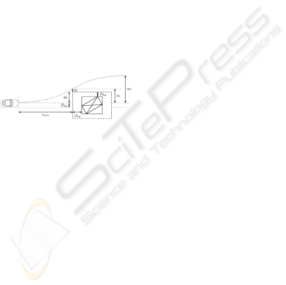
In Figure 5 the quantities necessary for the
calculation of the evasive trajectory are presented.
By means of the vehicle’s width b
v
and the
obstacle’s width the necessary evasive width y
A
is
determined together with a safety distance y
S
. Since
the evasive width can be reached before the end of
the maneuver, an associated maneuver width y
M
arises.
Figure 5: Evasive Quantities for calculating the evasive
trajectory (see text for details).
However, the evasive trajectory is the trajectory
until the evasive width y
A
is reached. The maneuver
width is chosen according to the strategy used. If the
maneuver width y
M
is chosen to be the same as the
evasive width y
A
, the evasive trajectory length s
steer
reaches its maximum for given maximal lateral
acceleration and maximal lateral jerk. These two
last-named parameters also determine the optimal
maneuver width which leads to the smallest possible
evasive trajectory length s
steer
and which makes use
of the set limits ideally. However, it needs
considerably more lateral offset for the same evasive
width y
A
.
6 LATERAL VEHICLE
GUIDANCE
If a collision with an obstacle is no longer avoidable
by a reaction of the driver, then, according to the
situation, the driver assistance system selects one of
the intervention strategies described above. For the
realization of the chosen intervention either the
active steering and/or the electro hydraulic braking
system are used according to the maneuver. If a
braking maneuver should be carried out, the vehicle
is decelerated (Schorn et al., 2005) by utilization of
the maximum force transmission available. The anti-
lock braking system ABS supports in this case.
In case a collision can only be prevented by an
evasive maneuver or by a combined evasive and
braking maneuver the control block receives from
intervention planning a trajectory, see Figure 1. The
vehicle is driven on this trajectory automatically
around the obstacle. Different linear and nonlinear
feedback controllers for an evasive maneuver were
developed, see e.g. (Schorn and Isermann, 2006),
(Schorn et al., 2006). Each lateral guidance feedback
control transfers an additional steering angle to the
interface of the steering system. Vehicle variables,
which cannot be measured directly by sensors the
vehicle is equipped with, are estimated, see Figure 1,
see also (Schorn and Isermann, 2006), (Isermann,
2006). For combined steering and braking
maneuvers different feedback controllers were
developed as well.
In the following only the lateral vehicle guidance
is regarded. Exemplarily, two of the investigated
approaches, a nonlinear asymptotic output tracking
feedback control and a speed-dependent local linear
feedback control approach with feedforward control
are presented.
6.1 Nonlinear Asymptotic Output
Tracking Feedback Control
For model based design of a feedback system, the
system behavior is required. The path following
feedback control is based on an extended one-track
model:
()
1111122
11
2211222
21
331 14
42
sin
0
0
xaxax
b
xaxax
b
u
xa xx
xx
⋅+ ⋅
⎡⎤⎡ ⎤
⎡⎤
⎢⎥⎢ ⎥
⎢⎥
⋅+ ⋅
⎢⎥⎢ ⎥
⎢⎥
=
+⋅
⎢⎥⎢ ⎥
⎢⎥
⋅+
⎢⎥⎢ ⎥
⎢⎥
⎢⎥
⎢⎥⎢ ⎥
⎣⎦
⎣⎦⎣ ⎦
&
&
&
&
(10)
[
]
E3
0010
y
yx
=
=⋅=x
(11)
with
1
2
3
E
4
()
()
and (t)
()
()
x
t
x
t
u
x
yt
x
t
β
ψ
δ
ψ
⎡⎤
⎡⎤
⎢⎥
⎢⎥
⎢⎥
⎢⎥
== =
⎢⎥
⎢⎥
⎢⎥
⎢⎥
⎢⎥
⎢⎥
⎣⎦
⎣⎦
x
&
(12)
β
is the sideslip angle,
ψ
the yaw angle, y
E
the
lateral vehicle position and
δ
the steer angle. The
speed dependent parameters follow from front and
rear cornering stiffness c
α
F
and c
α
R
, length from
ICINCO 2008 - International Conference on Informatics in Control, Automation and Robotics
38
front and rear axle to the center of gravity l
F
and l
R
,
velocity v, mass m and moment of inertia J
Z
, see
e.g., (Isermann, 2006):
FR RRFF
11 12
2
22
RRFF RRFF
21 22
ZZ
31
FFF
11 21
Z
1
cc lclc
aa
mv mv
lc lc lc lc
aa
JJv
av
ccl
bb
mv J
αα α α
αα α α
αα
+⋅−⋅
=− = −
⋅⋅
⋅−⋅ ⋅+⋅
==−
⋅
=
⋅
==
⋅
(13)
The model parameters were determined from
construction data and identification experiments,
(Schorn, 2007).
The lateral position y
E
(t)=f(x
E
(t)) of the vehicle
in an earth-fixed coordinate system has to be
controlled using the evasive trajectory described by
equation (5). The reference input of the control
system y
R
(t) is calculated by performing an
interpolation.
The vehicle model in (10) and (11) is a nonlinear
single-input single-output model of type:
00
() ( ) ( ) ()
( ) ( ( )) with ( )
tut
tt t
=+⋅
==
xaxbx
ycx xx
&
(14)
Having the system's output
y(t) converging
asymptotically to a prescribed reference output y
R
(t),
the system input u(t) can be calculated as follows
(Isidori, 1989), (Schwarz, 1999):
1
() 1 (1)
R1 R
1
1
()
LL ( )
L() () L () ()
d
d
dd i i
i
i
ut
c
cyt cyt
α
−
−−
−
=
=⋅
⎡⎤
−+−⋅ −
⎡
⎤
∑
⎣
⎦
⎢⎥
⎣⎦
ba
aa
x
xx
(15)
The relative degree d has to be determined according
to (Isidori, 1989), (Schwarz, 1999). For the
mentioned plant it yields d = 2 assuming v > 0 and
()
,...
2
3
,
2
41
ττ
±±≠+ xx . With this information, the
feedback control, equation (15), can be calculated.
The elements are given by (Schorn et al., 2006):
()
()( )
()
3
14
2
14 1111222
11 1 4
()
L() sin
L() cos
LL ( ) cos
cx
cvxx
cvxxaxaxx
cbv xx
=
=⋅ +
=− ⋅ + ⋅ + +
=⋅⋅ +
a
a
ba
x
x
x
x
(16)
where L
a
are so called Lie-functions (Isidori, 1989),
(Schwarz, 1999). The structure of the resulting
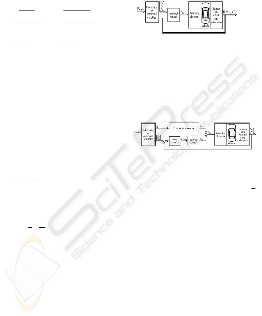
closed control loop is shown in Figure 6. The
command variables, the reference output y
R
(t),
(),
R
yt
&
()
R
yt
&&
as described above, are calculated in
the component “Calculation of command variables”.
The sideslip angle was estimated with a vehicle state
estimator (Schorn and Isermann, 2006). The output
of the controller is an additional steering
angle
)()(
M
tt
δ
δ
= .
Results from test drives with the experimental
vehicle described above will be presented below.
Figure 6: Structure of nonlinear asymptotic output
tracking feedback control.
6.2 Speed-dependent Local Linear
Feedback Control with
Feedforward Control
To guide a vehicle on a desired trajectory, a speed-
dependent local linear feedback control approach
with feedforward control was developed (Schorn
and Isermann, 2006). A scheme of the control
system is shown in Figure 7.
Figure 7: Structure of linear feedback control combined
with feedforward action.
Based on the self steer gradient SG a steer angle
δ
FF
is calculated for the feedforward control by means of
vehicle velocity v, wheelbase l and curvature
R
1
=
κ
of the desired trajectory:
(
)
2
FB
lSGv
δ
κ
=
+⋅⋅
(17)
A feedback control is added to compensate
disturbances and deviations. The parameters of a
proportional-derivative (PD) controller is tuned by
two parameters only and provides the required
dynamics by means of the differential component.
Using the vehicle orientation
ψ
, the control
deviation is transformed from an earth-fixed
coordinate system into a vehicle-fixed coordinate
system as control deviation e=
Δ
y. The feedback of
the vehicle’s longitudinal position
E
x
is necessary
for this purpose. The steering system is driven by the
sum
δ
M
of the angles
δ
FF
and
δ
FB
of the feedforward
and feedback control. For the implementation of the
feedback control in the experimental vehicle the
derivative, required for the calculation of the
differential component of the control variable, was
replaced by a high pass filter.
As the velocity v influences the vehicle’s
dynamics, because it changes continuously during a
COLLISION AVOIDANCE SYSTEM PRORETA - Strategies Trajectory Control and Test Drives
39
driving cycle. The feedback controllers were
designed for different operating points (velocities).
Their outputs are weighted and superimposed based
on Local Linear Models (LLM) (Schorn and
Isermann, 2006), (Nelles, 2001).
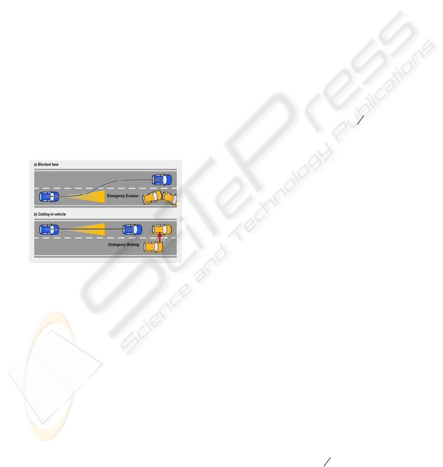
7 EXPERIMENTAL RESULTS
FROM TEST DRIVES
The developed components environment
recognition, intervention decision and feedback
control were implemented as a whole system in a
test vehicle and tested by means of numerous
experiments. This happened using an obstacle that
represents the rear view of a car and can be moved
laterally on the lane. Two test scenarios can be seen
in Figure 8.
In the following sections the most important
results from these tests are presented. It is required
in each case that the lateral and back lane areas are
monitored by additional sensors and thus permit
driving maneuvers.
Figure 8: Scenarios for practice system testing.
7.1 Blocked Lane
In the scenario "Suddenly appearing obstacle /
blocked lane" from Figure 8a) a lane is blocked
unexpectedly. An example for this would be an end
of a traffic jam in the case of bad visibility or after a
curve. The emergency evasion is then conducted as
an automatic intervention. The position of the used
obstacle is determined by the environmental sensors
and the necessary evasive trajectory is calculated
based on the information about the vehicle’s
surroundings. The vehicle is then guided aside of the
obstacle on the predefined evasive trajectory by the
lateral guidance controller without the assistance of
the driver.
Figure 9 shows results of a test drive with the
test vehicle mentioned above, where the asymptotic
nonlinear output tracking feedback control was
used. A comparison of desired command variable
and measured position shows that both values match
very well. The evasive width y
M
is 3m, the desired
and the actual position correspond well, apart from a
slight overshooting. The steering wheel angle
indicates that the driver held the steering wheel in a
straight position. The difference between total angle
and steering wheel angle is provided only by the
controller. The difference at the end of the
intervention maneuver follows from the fact that the
feedback control has been switched off at very low
velocities.
Results from test drives for the linear feedback
control combined with feedforward are presented in
Figure 10.
Again, desired command variable and measured
position match very well. The general conditions for
this test drive have been the same as for the results
shown in Figure 9 regarding evasive width y
M
and
velocity. The experiments show that the maximal
lateral accelerations are
2
7
m
y
s
a ≈
and the linear
controller needs less maximal steering angle. Both
control approaches presented above provide similar
accuracies, but the speed dependent linear control
system can be implemented and parameterized
easier and with smaller computational expense.
7.2 Cutting-in Vehicle
As a second scenario a suddenly cutting-in vehicle is
reproduced by moving the dummy obstacle just in
front of the vehicle from the right to the left lane
(Figure 8b). Evasion is not possible since further
obstacles block the right. The necessary maneuver is
thus an emergency braking maneuver. By means of
the environmental sensors it is recognized that both
lanes of the road are blocked and it is calculated at
which last possible moment the emergency braking
maneuver must be started in order to come to a stop
just before the obstacle. Assuming a maximum
braking acceleration which is dependent on the road
state (dry-wet), the required braking distance of the
vehicle is calculated depending on the current speed.
The driver assistance system triggers a braking
intervention only if this minimal braking distance is
reached in order to give the driver the chance to
prevent the collision as long as possible by himself.
The electro hydraulic braking system then
decelerates the vehicle maximally with support by
the anti-lock braking system ABS, on dry roads with
a deceleration of
2
10
m
x
s
a ≈
.
ICINCO 2008 - International Conference on Informatics in Control, Automation and Robotics
40
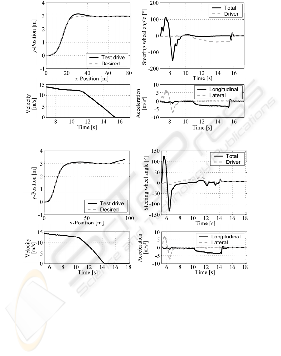
Figure 9: Results for asymptotic nonlinear output tracking feedback (test drive).
Figure 10: Results for linear feedback control combined with feedforward (test drive).
8 CONCLUSIONS
The described system for accident avoidance which
was developed within the scope of the project
PRORETA was presented to an audience selected by
Continental Teves and TU Darmstadt. The guests
had the possibility of experiencing the system within
the scope of driving experiments. Every guest drove,
amongst others, the scenarios presented in Figure 8.
The system worked robustly and faultlessly.
However, until such a system is available on the
market, some tasks have still to be solved. An
important one is the analysis of the oncoming traffic
which is examined in a subsequent PRORETA
project.
ACKNOWLEDGEMENTS
The authors highly appreciate the financial support
for the PRORETA project and good cooperation
with Continental Automotive Systems and the
support especially by Dr. R. Rieth, J. Diebold, M.
Arbitmann, Dr. S. Lüke, B. Schmittner. We also
COLLISION AVOIDANCE SYSTEM PRORETA - Strategies Trajectory Control and Test Drives
41

would like to thank our colleagues within the
PRORETA Team, Eva Bender and Michael Darms
with Prof. Winner, Prof. Landau and Prof. Bruder
for the excellent cooperation. Their results are
published e.g. in (Darms and Winner, 2006),
(Bender et al., 2006).
REFERENCES
Ameling, C., 2002. Steigerung der aktiven Sicherheit von
Kraftfahrzeugen durch ein Kollisionsvermeidungs-
system. VDI Verlag, Düsseldorf.
Bender, E., Darms, M., Schorn, M., Stählin, U., Isermann,
R., Winner, H., Landau, K.. 2007, Anti collision
system PRORETA - on the way to the collision
avoiding vehicle. Part 1: Basics of the System & Part
2: Results. ATZ (Automobiltechnische Zeitschrift,
English Supplement) 109 (4 & 5) 336-341 & 456-463.
Bender, E., Landau, K., 2006. Fahrerverhalten bei
automatischen Brems- und Lenkeingriffen eines
Fahrerassistenzsystems zur Unfallvermeidung, VDI-
Bericht 1931, AUTOREG 2006, Wiesloch.
Bender, E.; Landau, K., Bruder, R., 2006. Driver reactions
in response to automatic obstacle avoiding
manoeuvres. In: IEA 2006 – 16th World Congress on
Ergonomics, July 10-14, 2006, Maastricht, the
Netherlands.
Darms, M., 2007. Eine Basis-Systemarchitektur zur
Sensordatenfusion von Umfeldsensoren für
Fahreassistenzsysteme. Dissertation. Fortschr.-Ber.
Reihe 12, No. 653. VDI-Verlag, Düsseldorf.
Darms, M., Winner, H., 2006. Umfelderfassung für ein
Fahrerassistenzsystem zur Unfallvermeidung, VDI
Bericht 1931, AUTOREG 2006, Wiesloch.
Isermann, R., 1989. Digital control systems. Springer-
Verlag, Berlin and New York.
Isermann, R. (ed), 2006. Fahrdynamik-Regelung,
ATZ/MTZ-Fachbuch, Vieweg, Wiesbaden.
Isidori, A., 1989. Nonlinear Control Systems – An
Introduction. Springer-Verlag. Berlin.
Nelles, O., 2001. Nonlinear System Identification.
Springer-Verlag. Berlin.
Schorn, M., 2007. Quer- und Längsregelung eines
Personenkraftwagens für ein Fahrerassistenzsystem zu
Unfallvermeidung. Dissertation. Fortschr.-Ber. VDI
Reihe 12, no 651. VDI Verlag, Düsseldorf.
Schorn, M., Schmitt, J., Stählin, U., Isermann, R., 2005.
Model-based braking control with support by active
steering. In: 16th IFAC World Congress, July 4-8,
2005, Prague, Czech Republic.
Schorn, M., Isermann, R., 2006. Automatic Steering and
Braking for a Collision Avoiding Vehicle. 4th IFAC-
Symposium on Mechatronic Systems, September 12-
14, Wiesloch / Heidelberg.
Schorn, M., Stählin, U., Khanafer, A., Isermann, R., 2006.
Nonlinear Trajectory Following Control for Automatic
Steering of a Collision Avoiding Vehicle. American
Control Conference, June 14-16, Minneapolis,
Minnesota, USA.
Schwarz, H., 1999. Einführung in die Systemtheorie
nichtlinearer Regelungen. Shaker Verlag. Aachen.
Stählin, U., Schorn, M., Isermann, R., 2006.
Notausweichen für ein Fahrerassistenzsystem zur
Unfallvermeidung, VDI Bericht 1931, AUTOREG
2006, Wiesloch.
ICINCO 2008 - International Conference on Informatics in Control, Automation and Robotics
42
