
SENSOR AND ACTUATOR FAULT ANALYSIS IN ACTIVE
SUSPENSION IN VIEW OF FAULT-TOLERANT CONTROL
Claudio Urrea and Marcela Jamett
Departamento de Ingeniera El´ectrica, Av. Ecuador 3519, Est. Central, Santiago, Chile
Keywords:
Active suspension, sensor and actuator faults, full-vehicle suspension model.
Abstract:
This paper shows the first step of a fault tolerant control system (FTCS) to control active suspension on a
full-car suspension model. In this paper, the elimination of the inevitable pitch and roll actions of a spring
suspension between each axle and the body of a vehicle is studied. An actuator (linear motor) producing an
electromagnetic force and a pneumatic force acting simultaneously on the same output element is used. This
linear motor acts as a force generator that compensates instantly for the disturbing effects of the road surface.
Simulation results to illustrate the system’s performance in front of the occurrence of sensor and actuator faults
are shown.
1 INTRODUCTION
Vehicle suspension systems have developed over the
last 100 years to a very high level of sophistication
(Buckner, Schuetze, and Beno, 2000; Fukao, Ya-
mawaki, and Adachi, 2000). Most vehicle today use
a passive suspension system employing some type of
springs in combination with hydraulic or pneumatic
shock absorbers, and linkages with tailored flexibility
in various directions. These suspension system de-
signs are mostly based on ride analysis.
Traditionally automotive suspension designs have
been a compromise between the three conflicting cri-
teria of road holding, load carrying and passenger
comfort. In fact, despite the wide range of designs
currently available by using passive components, we
can only offer a compromise between these conflict-
ing criteria by providing spring and damping coeffi-
cients with fixed rates
1
.
On the other hand, active suspensions have been
extensively studied in the last three decades (Giua,
Seatzu, and Usai, 2000; Lefebvre, Chevrel,and
Richard, 2001; Lakehal-Ayat, Diop, and Fe-
naux,2002). In an active suspension the interaction
between vehicle body and wheel is regulated by an
actuator of variable length capable of supplying the
entire control force system’s requirements.
Ride comfort in ground vehicles usually depends
1
Components for passive suspension can only store and
dissipate energy in a pre-determined manner.
on a combination of vertical motion (heave) and an-
gular motion (pitch and roll). Active suspension is
characterized by a built-in actuator which can gen-
erate control forces to suppress the above mentioned
roll and pitch motions.
Including the dynamics of the hydraulic system
consisting of fluids, valves, pumps, etc., complicates
the active suspension control problem even further
since it introduces nonlinearities to the system. It
has been noted that the hydraulic dynamics and fast
servo-valve dynamics make controls design very dif-
ficult (Karlsson, Teely, and Hrovatz, 2001; Alleyne,
and Hedrick, 1995). The actuator dynamics signif-
icantly change the vibrational characteristics of the
vehicle system (Engelman, and Rizzon, 1993). Us-
ing a force control loop to compensate for the hy-
draulic dynamics can destabilize the system (Alleyne,
Liu, and Wright, 1998). This full nonlinear control
problem of active suspensions has been investigated
using several approaches including optimal control
based on a linearized model (Engelman, and Riz-
zon, 1993), adaptive nonlinear control (Alleyne, and
Hedrick, 1995), and adaptive control using backstep-
ping (Karlsson, Teely, and Hrovatz, 2001). These
schemes use linear approximations for the hydraulic
dynamics or they neglect the servo-valve model dy-
namics in which a current or voltage is what ulti-
mately controls the opening of the valve to allow flow
of hydraulic fluid to or from the suspension system.
However, nowadays a novel family of highly dynamic
electro-magnetic direct drives exit, i.e. servomotors
179
Urrea C. and Jamett M. (2008).
SENSOR AND ACTUATOR FAULT ANALYSIS IN ACTIVE SUSPENSION IN VIEW OF FAULT-TOLERANT CONTROL.
In Proceedings of the Fifth International Conference on Informatics in Control, Automation and Robotics - ICSO, pages 179-186
DOI: 10.5220/0001490201790186
Copyright
c
SciTePress
that looks like a hydraulic piston with acceleration
rates of over 200 [m/s
2
] make cyclic movement at
several Hertz possible.
Active suspension control systems reduce undesir-
able effects by isolating car body motion from vibra-
tions at the wheels, but their componentfailures/faults
are inevitable and unpredictable, and without care-
ful and prompt treatment, they tend to develop into
the severe total failure of the whole system. Conti-
nued operation of these systems has both economic
and safety implications. Every mechanical system is
vulnerable to faults that can lead to failure of the com-
plete system, unless mitigating strategies are included
at the design stage (Noura, Theilliol, and Sauter,
2000). Control element failures not only degrade the
performance of control systems, but also may intro-
duce instability and thus can cause serious operation
and safety problems. Therefore, fault tolerance has
been one of the major issues in process control.
In automated systems, the goal of the fault-
tolerance is to continue operation in spite of failures,
if this is possible. A general problem has been that
fault conditions could not be treated as an integrated
part of system design. Therefore, automated systems
to provide uninterrupted service, even in the presence
of failures are required (Zhang, Jiang, 2002).
Most of the past work uses the quarter-car model,
which includes only two degree-of-freedomof the ve-
hicle motion in the vertical direction (Lakehal-Ayat,
Diop, and Fenaux,2002). In general, the heave, pitch
and roll motions are coupled and an impulse at the
front or rear wheels excites all three motions. This
means that pitch-, heave- and roll-controllers can-
not be independently designed. Therefore, we take
a model based in (Ikenaga, Lewis, Campos, Davis,
2000) including the full vehicle suspension dynamics
considering heave, pitch and roll motions.
The paper is organized as follows: in section 2 the
system description is given. In section 3, the state-
space model for the full-vehicle suspension model is
presented. In section 4, the vehicle controller is de-
veloped. Section 5 presents fault analysis and some
simulation results. Finally, in section 6, the conclu-
sions and outline future work are discussed.
2 SYSTEM DESCRIPTION
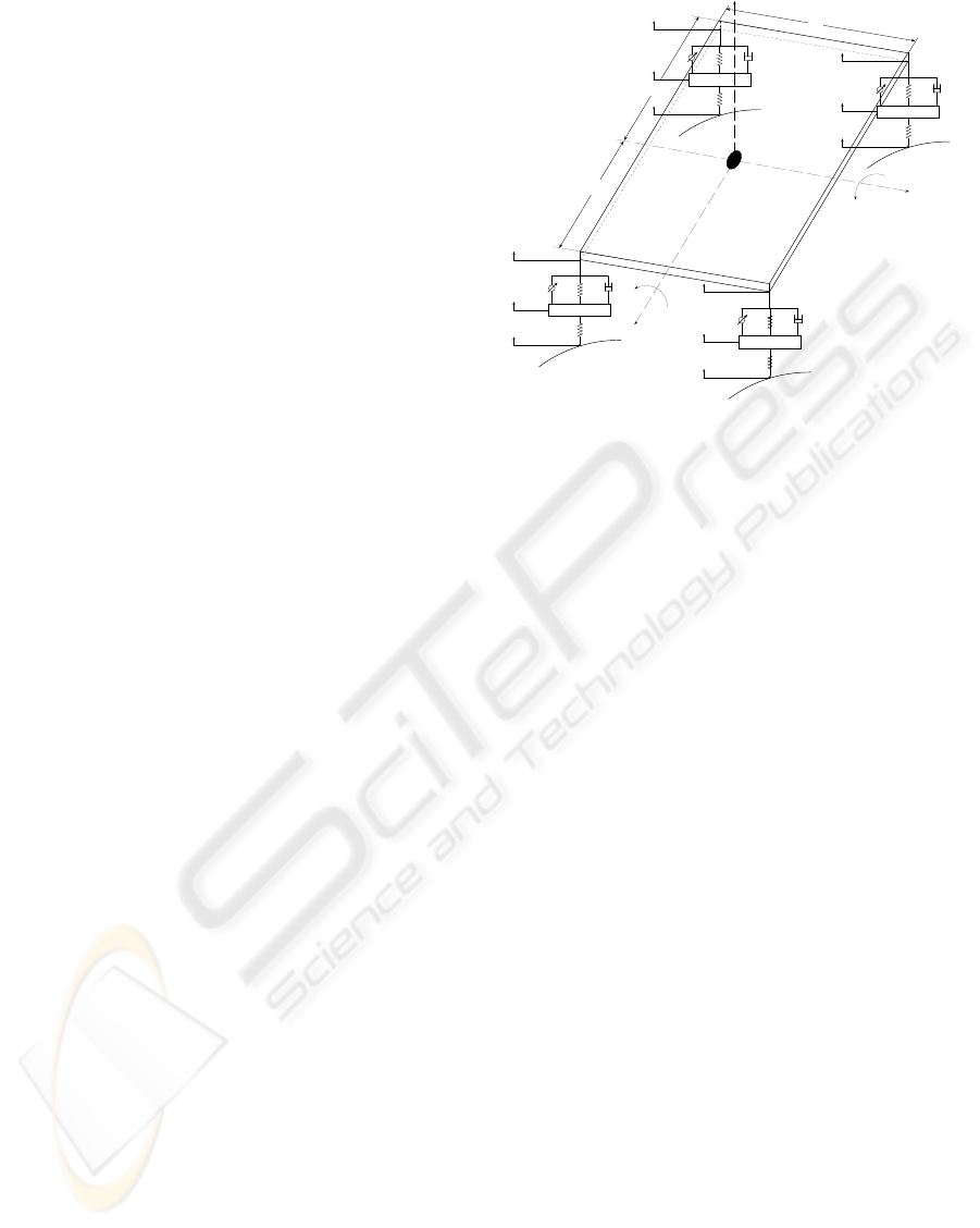
2.1 Full-Vehicle Suspension Model
(Seven DOF System)
In this work, a full-vehicle suspension mathematical
model depicted in Fig.1 is considered.
F
fl
ks
fl
Bs
fl
ku
fl
mu
fl
zr
fl
zu
fl
zs
fl
F
rl
ks
rl
Bs
rl
ku
rl
mu
rl
zr
rl
zu
rl
zs
rl
F
rr
ks
rr
Bs
rr
ku
rr
mu
rr
zr
rr
zu
rr
zs
rr
F
fr
ks
fr
Bs
fr
ku
fr
mu
fr
zr
fr
zu
fr
zs
fr
ϕ
Z
ms
Y
X
θ
b
w
a
Figure 1: Full-vehicle suspension model.
where the followings parameters and variables are
taken which respect to the static equilibrium position
(Ikenaga, Lewis, Campos, Davis, 2000):
• ms is sprung mass [kg],
• mu is unsprung mass [kg],
• Ks
fl
is front-left suspension spring stiffness
[N/m],
• Ks
fr
is front-right suspension spring stiffness
[N/m],
• Ks
frl
is rear-left suspension spring stiffness
[N/m],
• Ks
rr
is rear-right suspension spring stiffness
[N/m],
• Bs
fl
is front-left suspension damping [N/m/s],
• Bs
fr
is front-right suspension damping [N/m/s],
• Bs
frl
is rear-left suspension damping [N/m/s],
• Bs
rr
is rear-right suspension damping [N/m/s],
• Ku
fl
is tire-left spring stiffness [N/m],
• Ku
fr
is tire-right spring stiffness [N/m],
• Ku
frl
is tire-left spring stiffness [N/m],
• Ku
rr
is tire-right spring stiffness [N/m],
• a is length between front of vehicle and center of
gravity of sprung mass [m],
• b is length between rear of vehicle and center of
gravity of sprung mass [m],
• w is width of sprung mass [m],
• I
xx
is roll axis moment of inertia [kg · m
2
],
• I
yy
is pitch axis moment of inertia [kg · m
2
],
ICINCO 2008 - International Conference on Informatics in Control, Automation and Robotics
180
• F
fl
is force at the front-left suspension [N],
• F
fr
is force at the front-right suspension [N],
• F
rl
is force at the rear-left suspension [N],
• F
rr
is force at the rear-right suspension [N],
• Zr
fl
is terrain disturbance heights at the front-left
wheel [m],
• Zr
fr
is terrain disturbance heights at the front-
right wheel [m],
• Zr
rl
is terrain disturbance heights at the rear-left
wheel [m],
• Zr
rr
is terrain disturbance heights at the rear-right
wheel [m],
• g is the constant of graveness in the terrestrial sur-
face, 9.80665 [m/s
2
].
In this model, the car body is represented as a
sprung mass, and the wheels are represented as an
unsprung mass connected to the ground via the tire
spring. The tire is an undamped spring between the
axle and the ground. The suspension consists of pas-
sive dampers in parallel with four actuators and four
springs.
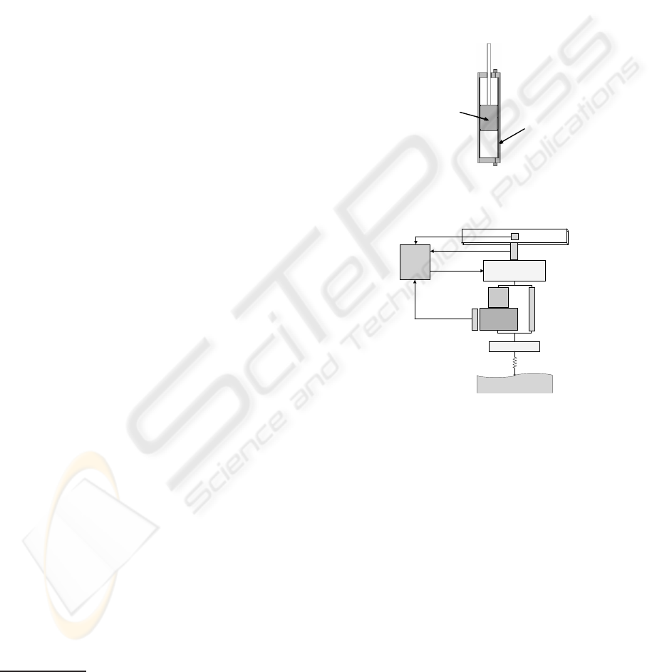
2.2 Actuators
The suspension actuators are taken to be a force actu-
ator acting between the car body and the axle of the
car. The chosen ServoRam
TM2
actuator, depicted in
Fig. 2, produces an electromagnetic force and a pneu-
matic force acting simultaneously on the same output
element. This electromagnetic actuator has zero me-
chanical hysteresis, since the force is applied directly
to the output element. It has zero electrical hystere-
sis because a microamp in one direction produces a
positive force, and a microamp in the opposite direc-
tion produces a negative force, so that the force output
is an exactly linear function of the current input. A
linear transducer measures the position of the piston.
The small control time constant allows the force to
be changed at a rate of thousands of Newtons per mil-
lisecond, so the suspension system can instantly adapt
to every road condition. These linear motors consists
of just two parts: the fixed stator and the moveable
slider. These two parts are not connected by slip rings
or by cables. Since the linear stroke directly with-
out the use of mechanical gears, belts or ball screws,
there is no wear or mechanical play. In a practical
point of view, the ram is placed between the wheel
2
Name applied to the AMTr ram technology, and all
AMTr electromagnetic rams are, in fact, ServoRam
TM
.
This technology has been developed over the last 10 years
by AMT’s Chief Scientist, Phillip Denne.
point (on the vehicle chassis) and the wheel stub axle,
so as to carry all the vertical forces, see Fig. 3. The
forces transferred from the wheel to the chassis may
be precisely controlled by the electromagnetic forces.
A force-measuring transducer may be used to control
the current to the coil system, so as to maintain the
total upward force at a constant value, irrespective of
the wheel vertical motion. The desired value of this
constant force may be determined in turn by the out-
put from a wheel-point accelerometer, so as to hold
the vehicle steady against pitch and roll motions, for
example.
Magnet array on moving
armature/piston
Coil array on fixed
stator/cylinder
Figure 2: Simplified schematic of the ServoRam
TM
actua-
tor.
k
u
m
u
Ground
Electromagnetic
forces
Acceleremeter
Correction
Force
control
loop
force transducer
Ram position
transducer
friction
Suspension
mass
Air
Spring
Figure 3: ServoRam
TM
actuator system for active suspen-
sion.
3 STATE SPACE-MODEL
The governing equations of this system are presented
considering the following state variables (Ikenaga,
Lewis, Campos, Davis, 2000):
• x
1
= z is the heave position (ride height of sprung
mass),
• x
2
= ˙z is the heave velocity (payload velocity of
sprung mass),
• x
3
= θ is the pitch angle,
• x
4
=
˙
θ is the pitch angular velocity,
• x
5
= φ is the roll angle,
• x
6
=
˙
φ is the roll angular velocity,
SENSOR AND ACTUATOR FAULT ANALYSIS IN ACTIVE SUSPENSION IN VIEW OF FAULT-TOLERANT
CONTROL
181

• x
7
= Zu
fl
is the front-left wheel unsprung mass
height,
• x
8
=
˙
Zu
fl
is the front-left wheel unsprung mass
velocity,
• x
9
= Zu
fr
is the front-right wheel unsprung mass
height,
• x
10
=
˙
Zu
fr
is the front-right wheel unsprung mass
velocity,
• x
11
= Zu
rl
is the rear-left wheel unsprung mass
height,
• x
12
=
˙
Zu
rl
is the rear-left wheel unsprung mass
velocity,
• x
13
= Zu
rr
is the rear-right wheel unsprung mass
height,
• x
14
=
˙
Zu
rr
is the rear-right wheel unsprung mass
velocity,
Linear differential equations that describe the dynam-
ics can be formulated as:
˙x
1
= x
2
˙x
2
= (F
fl
+ F
fr
+ F
rl
+ F
rr
− (Ks
fl
+ Ks
fr
+ Ks
rl
+Ks
rr
) · x
1
− (Bs
fl
+ Bs
fr
+ Bs
rl
+ Bs
rr
) · x
2
·
+(a· (Ks
fl
+ Ks
fr
) − b· (Ks
rl
+ Ks
rr
))x
3
+
(a· (Bs
fl
+ Bs
fr
) − b· (Bs
rl
+ Bs
rr
)) · x
4
+
Ks
fl
· x
7
+ Bs
fl
· x
8
+ Ks
fr
· x
9
+ Bs
fr
· x
10
+
Ks
rl
· x
11
+ Bs
rl
· x
12
+ Ks
rr
· x
13
+ Bs
rr
· x
14
)
/ms− g
˙x
3
= x
4
˙x
4
= (−a· (F
fl
+ F
fr
) + b· (F
rl
+ F
rr
) + (a· (Ks
fl
+ Ks
fr
) − b· (Ks
rl
+ Ks
rr
)) · x
1
+ (a· (Bs
fl
+ Bs
fr
) − b· (Bs
rl
+ Bs
rr
)) · x
2
− (a
2
· (Ks
fl
+Ks
fr
) + b
2
· (Ks
rl
+ Ks
rr
)) · x
3
− (a
2
· (
Bs
fl
+ Bs
fr
) + b
2
· Bs
rl
+ Bs
rr
)) · (x
4
− a·
Ks
fl
· x
7
− a· Bs
fl
· x
8
− a· Ks
fr
· x
9
− a·
Bs
fr
· x
10
+ b· Ks
rl
· x
11
+ b· Bs
rl
· x
12
+ b·
Ks
rr
· x
13
+ b· Bs
rr
· x
14
)/I
yy
(1)
˙x
5
= x
6
˙x
6
= ((F
fl
− F
fr
+ F
rl
− F
rr
) −
w
2
· ((Ks
fl
+ Ks
fr
+ Ks
rl
+ Ks
rr
) · x
5
+ (Bs
fl
+ Bs
fr
+ Bs
rl
+
Bs
rr
)) · x
6
+ Ks
fl
· x
7
+ Bs
fl
· x
8
− Ks
fr
· x
9
−Bs
fr
· x
10
+ Ks
rl
· x
11
+ Bs
rl
· x
12
− Ks
rr
·
x
13
+ Bs
rr
· x
14
)/(2· w/I
xx
)
˙x
7
= x
8
˙x
9
= x
10
˙x
10
= (−F
fr
+ Ks
fr
· x
1
+ Bs
fr
· x
2
− a· Ks
fr
· x
3
−a· Bs
fr
· x
4
−
w
2
· Ks
fr
· x
5
−
w
2
· Bs
fr
· x
6
−(Ku
fr
+ Ks
fr
) · x
9
− Bs
fr
· x
10
+ Ku
fr
·
Zr
fr
)/mu
fr
− g
˙x
11
= x
12
˙x
12
= (−F
rl
+ Ks
rl
· x
1
+ Bs
rl
· x
2
+ b· Ks
rl
· x
3
+
b· Bs
rl
· x
4
+
w
2
· Ks
rl
· x
5
+
w
2
· Bs
rl
· x
6
−
(Ku
rl
+ Ks
rl
) · x
11
− Bs
rl
· x
12
+ Ku
rl
· Zr
rl
)
/mu
rl
− g
˙x
13
= x
14
˙x
14
= (−F
rr
+ Ks
rr
· x
1
+ Bs
rr
· x
2
+ b· Ks
rr
· x
3
+
b· Bs
rr
· x
4
−
w
2
· Ks
rr
· x
5
−
w
2
· Bs
rr
· x
6
−
(Ku
rr
+ Ks
rr
) · x
13
− Bs
rr
· x
14
+ Ku
rr
· Zr
rr
)
/mu
rr
− g (2)
This system can be summarized by the following lin-
ear space-state representation:
˙x(t) = A· x(t) + B· u(t) + B
p
· u
p
(t)
y(t) = C· x(t), (3)
where:
• x ∈ ℜ
14x1
is the system state vector,
• u ∈ ℜ
4x1
is a vector composed of the control
forces. u = [F
fl
F
fr
F
rl
F
rr
]
T
,
• u
p
∈ ℜ
5x1
is a vector whose components are the
disturbance inputs. u
p
= [g Zr
fl
Zr
fr
Zr
rl
Zr
rr
]
T
,
• y ∈ ℜ
3x1
is the system output vector. y = [Z θ ϕ]
T
,
• A,B,B
p
,and C are constant matrices of appropri-
ate dimensions.
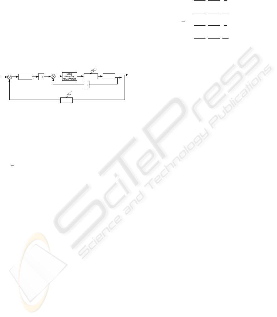
4 CONTROLLER MODEL
The controller design considers:
• Control loops that stabilize heave, pitch and roll
responses,
ICINCO 2008 - International Conference on Informatics in Control, Automation and Robotics
182
• Input decoupling transformation that blends the
inner and outer control loops allowing stream-
lined design yet gives performance better than
over-simplified decoupled techniques.
By employing a state observer, the full state feed-
back is available for the entire vehicle, and pitch an-
gle is inferred from a combination of rate sensors and
accelerometers. The control law ¯u is computed by
a state feedback associated with the integral of the
tracking error: ¯u = - [K
1
K
2
] · [x q]
T
= - K · ¯x; K
1
and
K
2
are computed according to Eq.4. This controller
design is illustrated in Fig.4.
Fault
System
y
x
+
+
- K
Integrator
+
-
x
d
Sensors
Fault
q
q
.
u
u
Actuators
- K
Figure 4: Controller block diagram.
The control procedure can be briefly summarized
as follows: Let us consider the followingoptimization
problem.
The performance index to be minimized is:
J =
1
2
·
Z
∞
0
[ ¯x
T
(t) · Q· ¯x(t) + ¯u
T
(t) · R· ¯u(t)]dt, (4)
where:
• ¯x ∈ ℜ
17x1
is the augmented system state vector. ¯x
= [x
T
q
T
]
T
,
• ¯u ∈ ℜ
3x1
is a vector whose components are the
control forces, provided by the actuators, for
heave (F
z
), pitch (F
θ
) and roll (F
ϕ
),
• Q ∈ ℜ
17x17
is positive semi-definite matrix,
• R ∈ ℜ
3x3
is tuning diagonal matrix.
The good performance of the suspension system
is related to the minimization of the term ¯x
T
·Q· ¯x and
an adequate choice of R, because the comfort depends
of the term ¯u
T
·R· ¯u. The optimal control strategy that
minimizes the cost function was found to be ¯u(t) =
- K· ¯x(t), where the gain matrix Kcan be computed
by solving an algebraic Riccati equation. So, a set
of LQR optimal feedback gains corresponding to dif-
ferent weighting factors in the quadratic function J is
chosen. The feedback control is designed to increase
the relative damping of a particular mode of motion
in the system by augmenting one or more of the co-
efficients of the equation of motion by actuating the
control signals in response to motion feedback vari-
ables.
From Fig.1, the equivalent relationship between
F
z
(t), F
θ
(t) and F
ϕ
(t), and the forces generated by the
actuators can be defined by:
F
fl
(t)
F
fr
(t)
F
rl
(t)
F
rr
(t)
=
1
2
b
(a+b)
−1
(a+b)
1
w
b
(a+b)
−1
(a+b)
−1
w
a
(a+b)
1
(a+b)
1
w
a
(a+b)
1
(a+b)
−1
w
·
F
z
(t)
F
θ
(t)
F
ϕ
(t)
,
(5)
Therefore the nominal control is given by:
F
z
(t)
F
θ
(t)
F
ϕ
(t)
= − K · ¯x(t), (6)
where K ∈ ℜ
3x17
.
5 FAULT ANALYSIS AND
SIMULATION RESULTS
In the following simulations, the full-car suspension
system was simulated for the input terrain distur-
bances Zr(t) actuating between 2 ≤ t ≤ 8 s:
Zr(t) =
Zr
fl
(t)
Zr
fr
(t)
Zr
rl
(t)
Zr
rr
(t)
=
0.05· sin(w·t)
0.15· sin(w·t)
0.05· sin(w· (t +τ))
0.15· sin(w· (t +τ))
, (7)
where:
• ω = 9 [rad/s], is the terrain disturbance frequency,
• τ = 0.1409 [s], is the time delay given by: τ = L/v
= (a+ b)/v,
• L is the distance between the front and rear axles
of the vehicle [m],
• v = 22 [m/s], is the speed at which the vehicle
travels.
The given initial conditions are ¯x = 0, and the re-
quired torque to be delivered by the actuators is deter-
mined as in fault-free cases. The objective here is to
analyze the effects of a sensor- and actuator-faults on
the active suspension.
5.1 Sensor Fault
At t = 5.5 s a sensor fault occurs in the second sensor
measuring θ. This fault corresponds to a bias equal
SENSOR AND ACTUATOR FAULT ANALYSIS IN ACTIVE SUSPENSION IN VIEW OF FAULT-TOLERANT
CONTROL
183
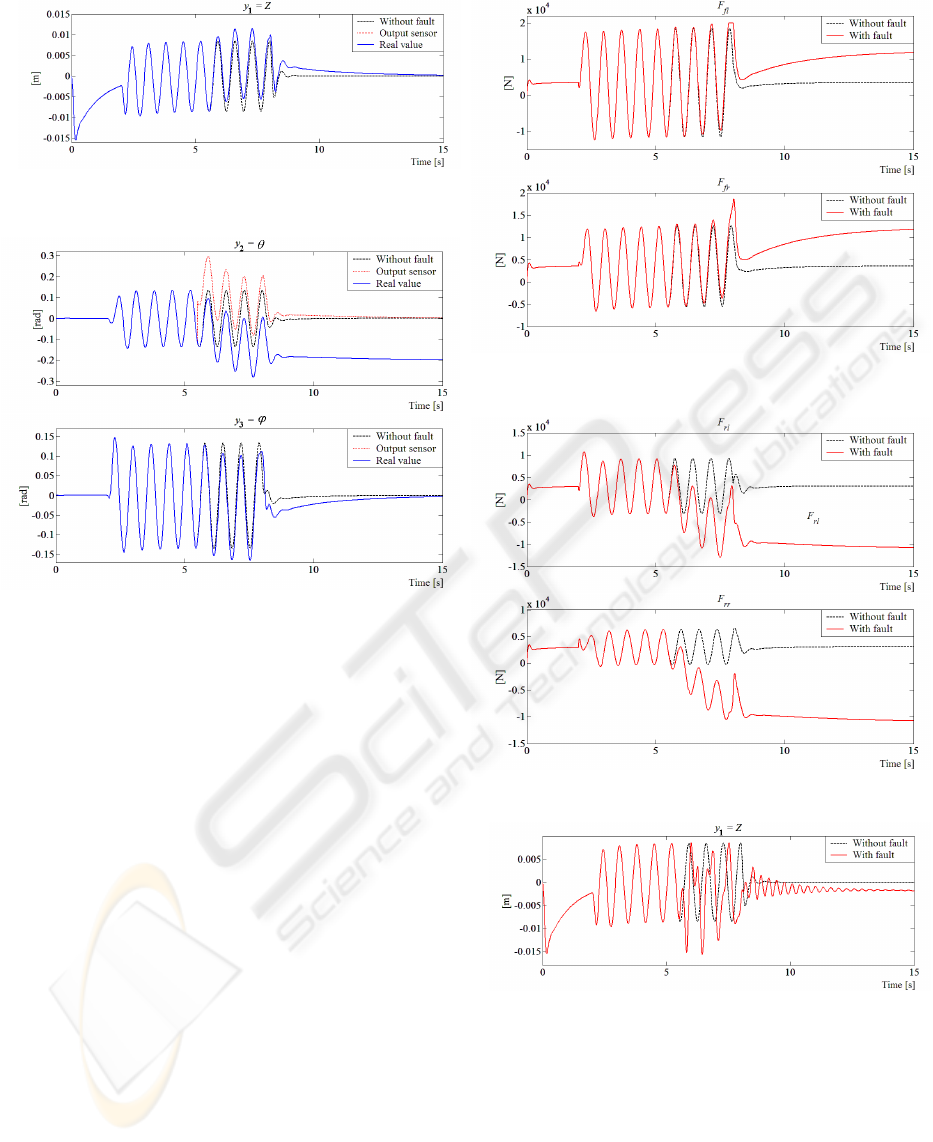
Figure 5: y
1
: Heave position (ride height of sprung mass).
Figure 6: (a) y
2
: Pitch angle; (b) y
3
: Roll angle.
to 0.2 rad. Due to this fault, similar real value θ is
shifted of - 0.2 rad from the output sensor which goes
to its reference value. The real value of θ is far from
its reference because the control input naturally reacts
in the presence of the sensor fault. Figs. 5 and 6 show
that the other outputs Z and ϕ are also affected by this
fault but reach their reference value again.
The increase of the necessary force that should be
applied to the actuators in front of this default is de-
picted in Figs. 7 and 8. Fig. 7(a) illustrates a satu-
ration (± 20000 [N]) reached in the actuator, in the
presence of this fault. Figs. 7(b) and 8 show the other
influence of this sensor fault on the control input.
5.2 Actuator Fault
Other experiments simulating actuator faults are per-
formed. At t = 5.5 [s], a reduction of 75% in the se-
cond actuator effectiveness (F
fr
) is simulated. Figs.
9 to 12. illustrate simulation results. Figs. 9 and 10
show the permanent shift between the outputs with
no fault and the outputs with fault. This shift is due
to the fact that the other control inputs are affected by
the fault due to the closed-loop and coupling between
each other.The new necessary forces that should be
applied in the actuators to compensate this loss of
Figure 7: (a) F
fl
: Force at the front-left suspension; (b) F
fr
:
Force at the front-right suspension.
Figure 8: (a) F
rl
: Force at the rear-left suspension; (b) F
rr
:
Force at the rear-right suspension.
Figure 9: y
1
: Heave position (ride height of sprung mass).
effectiveness are shown in Figs. 11 and 12. These
force increases do not surpass the maximum allow-
able force limits in the actuators.
ICINCO 2008 - International Conference on Informatics in Control, Automation and Robotics
184
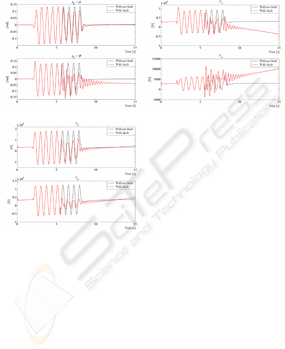
Figure 10: (a) y
2
: Pitch angle; (b) y
3
: Roll angle.
Figure 11: (a) F
fl
: Force at the front-left suspension; (b)
F
fr
: Force at the front-right suspension.
6 CONCLUSIONS AND FUTURE
WORK
In this paper, it was shown that active suspension can
improve all three performance aspects i.e. passenger
ride comfort, handling, and rattle space.
A nominal control law is designed for this active
suspension system and the effect of the profile of the
road is analyzed in the first part. The main aim of
this work is the study of the influence of sensor and
actuator faults on the control law.
The obtained results are realistic and show the im-
portance of the design of a fault tolerant control sys-
tem (FTCS) able to compensate this kind of fault.
This work is just starting. Future work will also take
into account the loss of a complete sensor or actuator
in order to preserve safety and passengers’ comfort.
Figure 12: (a) F
rl
: Force at the rear-left suspension; (b) F
rr
:
Force at the rear-right suspension.
ACKNOWLEDGEMENTS
This work was possible thanks to the support of DI-
CYT – Universidad de Santiago de Chile, USACH,
through Project 0607UO and Project 0607JD.
REFERENCES
Buckner G., Schuetze K., Beno J.: Active Vehicle Suspen-
sion Control Using Intelligent Feedback Lineariza-
tion. American Control Conference, Chicago, Illinois,
USA (2000) 4019–4024
Fukao T., Yamawaki A., Adachi N.: Nonlinear and H
∞
Con-
trol of Active Suspension Systems with Hydraulic Ac-
tuators. American Control Conference, Chicago, Illi-
nois, USA (2000) 5125–5128
Giua A., Seatzu C., Usai G.: ActiveAxletree Suspension for
Road Vehicles with Gain-Switching. 39th IEEE Con-
ference on Decision and Control Sydney Convention
and Exhibition Centre, Sydney, Australia (2000)
Lefebvre D., Chevrel P.,Richard S.: A Hinfinity-based con-
trol design methodology dedicated to active control of
vehicle longitudinal oscillations. 40th IEEE Confer-
ence on Decision and Control Orlando, Florida, USA
(2001) 99–104
Lakehal-Ayat M., Diop S., Fenaux E.: Development of a
Full Active Suspension System. 15th Triennial World
Congress IFAC, Barcelona, Spain (2002)
Karlsson N., Teely A., Hrovatz D.: A Backstepping Ap-
proach to Control of Active Suspensions. 40th IEEE
Conference on Decision and Control Orlando, Florida,
USA (2001) 4170–175
Alleyne A., Hedrick J.: Nonlinear Adaptive Control of Ac-
tive Suspensions. IEEE Trans. Control Syst. Technol.
1 (1995) 94–101
SENSOR AND ACTUATOR FAULT ANALYSIS IN ACTIVE SUSPENSION IN VIEW OF FAULT-TOLERANT
CONTROL
185

Engelman G., Rizzon G.: Including the Force Generation
Process in Active Suspension Control Formulation.
American Control Conference, San Francisco, Cali-
fornia, USA (1993)
Alleyne A., Liu R., Wright H.: On the Limitations of
Force Tracking Control for Hydraulic Active Suspen-
sions. American Control Conference, Philadelphia,
USA (1998) 43–47
Noura H., Theilliol D., Sauter D.: Actuator Fault-Tolerant
Control Design: Demostration on a Three-Tank-
System. International Journal of Systems Science se-
ries 9 (2000) 1143–1155
Zhang Y., Jiang J.: Design of Restructurable Active
Faut-Tolerant Control Systems. 15th Triennial World
Congress IFAC, Barcelona, Spain (2002)
Ikenaga S., F. Lewis, Campos J., Davis L.: Active
Suspension Control of Ground Vehicle Based on a
Full-Vehicle Model. American Control Conference,
Chicago, Illinois, USA (2000) 4019–4024
ICINCO 2008 - International Conference on Informatics in Control, Automation and Robotics
186
