
LEARNING BY EXAMPLE
Reinforcement Learning Techniques for Real Autonomous Underwater Cable
Tracking
Andres El-Fakdi, Marc Carreras
Computer Vision and Robotics Group (VICOROB), Institute of Informatics and Applications
University of Girona, 17074 Girona, Spain
Javier Antich, Alberto Ortiz
Department of Mathematics and Computer Science, University of Balearic Islands, 07071 Palma de Mallorca, Spain
Keywords:
Machine learning in control applications, space and underwater robots.
Abstract:
This paper proposes a field application of a high-level Reinforcement Learning (RL) control system for solving
the action selection problem of an autonomous robot in cable tracking task. The learning system is charac-
terized by using a Direct Policy Search method for learning the internal state/action mapping. Policy only
algorithms may suffer from long convergence times when dealing with real robotics. In order to speed up the
process, the learning phase has been carried out in a simulated environment and, in a second step, the policy
has been transferred and tested successfully on a real robot. Future steps plan to continue the learning process
on-line while on the real robot while performing the mentioned task. We demonstrate its feasibility with real
experiments on the underwater robot ICTINEU
AUV
.
1 INTRODUCTION
Reinforcement Learning (RL) is a widely used
methodology in robot learning (Sutton and Barto,
1998). In RL, an agent tries to maximize a scalar
evaluation obtained as a result of its interaction with
the environment. The goal of a RL system is to find
an optimal policy to map the state of the environ-
ment to an action which in turn will maximize the ac-
cumulated future rewards. The agent interacts with
a new, undiscovered environment selecting actions
computed as the best for each state, receiving a nu-
merical reward for every decision. The rewards are
used to teach the agent and in the end the robot learns
which action it must take at each state, achieving an
optimal or sub-optimal policy (state-action mapping).
The dominant approach over the last decade has
been to apply reinforcement learning using the value
function approach. Although value function method-
ologies have worked well in many applications, they
have several limitations. The considerable amount of
computational requirements that increase time con-
sumption and the lack of generalization among con-
tinuous variables represent the two main disadvan-
tages of ”value” RL algorithms. Over the past few
years, studies have shown that approximating a pol-
icy can be easier than working with value functions,
and better results can be obtained (Sutton et al., 2000)
(Anderson, 2000). Informally, it is intuitively sim-
pler to determine how to act instead of value of act-
ing (Aberdeen, 2003). So, rather than approximat-
ing a value function, new methodologies approximate
a policy using an independent function approxima-
tor with its own parameters, trying to maximize the
future expected reward. Only a few but promising
practical applications of policy gradient algorithms
have appeared, this paper emphasizes the work pre-
sented in (Bagnell and Schneider, 2001), where an
autonomous helicopter learns to fly using an off-line
model-based policy search method. Also important is
the work presented in (Rosenstein and Barto, 2001)
where a simple “biologically motivated” policy gra-
dient method is used to teach a robot in a weightlift-
ing task. More recent is the work done in (Kohl and
Stone, 2004) where a simplified policy gradient algo-
rithm is implemented to optimize the gait of Sony’s
AIBO quadrupedal robot.
All these recent applications share a common
drawback, gradient estimators used in these algo-
rithms may have a large variance (Marbach and Tsit-
siklis, 2000)(Konda and Tsitsiklis, 2003) what means
that policy gradient methods learn much more slower
61
El-Fakdi A., Carreras M., Antich J. and Ortiz A. (2008).
LEARNING BY EXAMPLE - Reinforcement Learning Techniques for Real Autonomous Underwater Cable Tracking.
In Proceedings of the Fifth International Conference on Informatics in Control, Automation and Robotics - RA, pages 61-68
DOI: 10.5220/0001490500610068
Copyright
c
SciTePress
than RL algorithms using a value function (Sutton
et al., 2000) and they can converge to local optima of
the expected reward (Meuleau et al., 2001), making
them less suitable for on-line learning in real appli-
cations. In order to decrease convergence times and
avoid local optimas, newest applications combine pol-
icy gradient algorithms with other methodologies, it
is worth to mention the work done in (Tedrake et al.,
2004) and (Matsubara et al., 2005), where a biped
robot is trained to walk by means of a “hybrid” RL al-
gorithm that combines policy search with value func-
tion methods.
One form of robot learning, commonly called
teaching or learning by example techniques, offers a
good proposal for speeding up gradient methods. In
those ones, the agent learns to perform a task by an-
alyzing or “watching” the task being performed by a
human or control code. The advantages of teaching
are various. Teaching can direct the learner to ex-
plore the promising part of search space which con-
tains the goal states. This is a very important aspect
when dealing with large state-spaces whose explo-
ration may be infeasible. Also, local maxima dead
ends can be avoidedwith example learning techniques
(Lin, 1992). Differing from supervised learning, bad
examples or “bad lessons” will also help the agent to
learn a good policy, so the teacher can also select bad
actions during the teaching period. The idea of pro-
viding high-level information and then use machine
learning to improve the policy has been successfully
used in (Smart, 2002) where a mobile robot learns
to perform a corridor following task with the supply
of example trajectories. In (Atkenson et al., 1997)
the agent learns a reward function from demonstra-
tion and a task model by attempting to perform the
task. Finally, cite the work done in (Hammer et al.,
2006) concerning an outdoor mobile robot that learns
to avoid collisions by observing a human driver oper-
ate the vehicle.
This paper proposes a reinforcement learning ap-
plication where the underwater vehicle ICTINEU
AUV
carries out a visual based cable tracking task using a
direct gradient algorithm to represent the policy. An
initial example policy is first computed by means of
computer simulation where a model of the vehicle
simulates the cable following task. Once the simu-
lated results are accurate enough, in a second phase,
the policy is transferred to the vehicle and executed in
a real test. A third step will be mentioned as a future
work, where the learning procedure continues on-line
while the robot performs the task, with the objective
of improving the initial example policy as a result of
the interaction with the real environment. This pa-
per is structured as follows. In Section 2 the learning
Supply policy
Environment
r
t
s
t
t
Learning
Algorithm
Supply policy
Environment
r
t
s
t
t
Learning
Algorithm
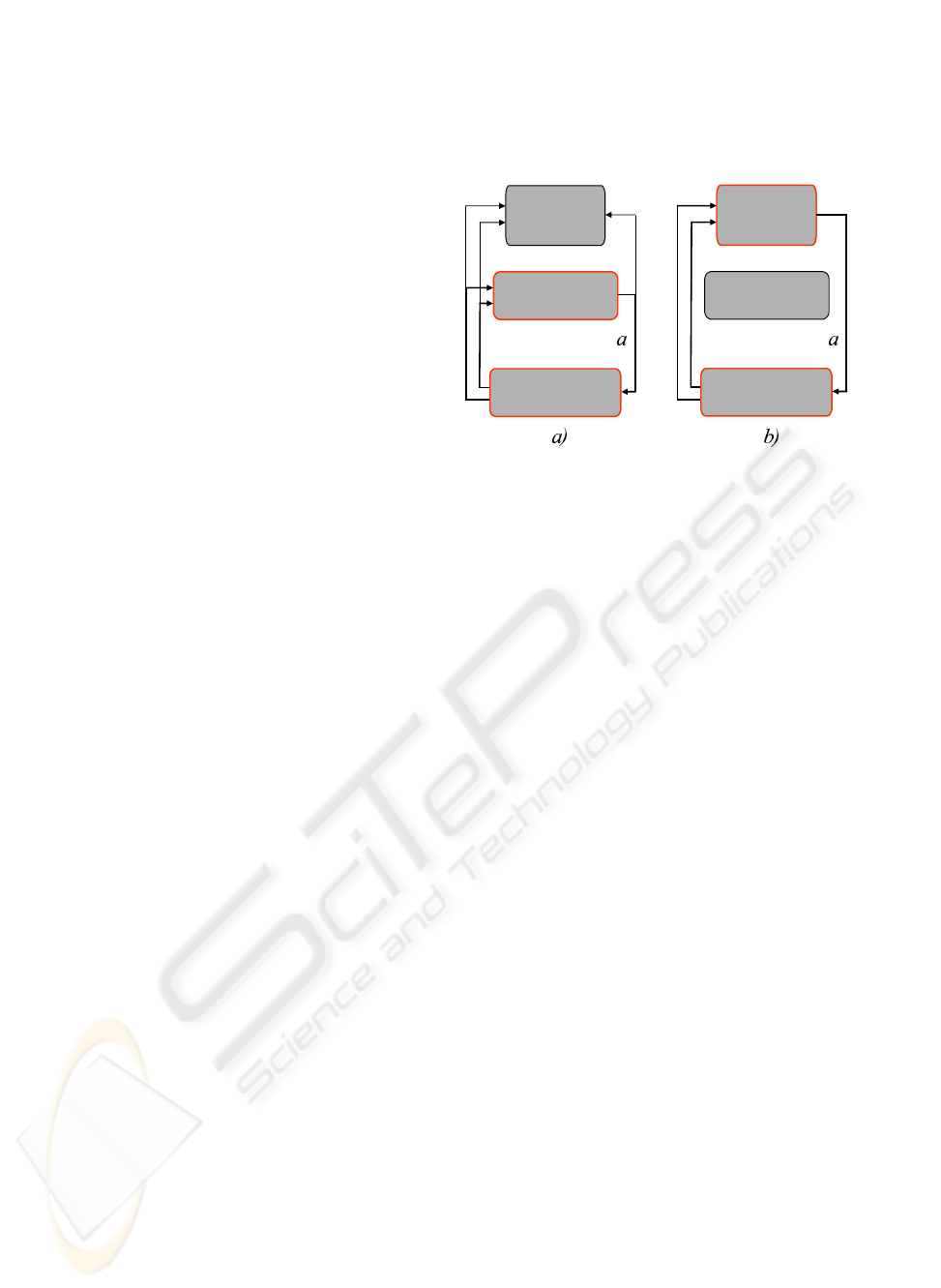
Figure 1: Learning phases.
procedure and the policy gradient algorithm are de-
tailed. Section 3 describes all the elements that affect
our problem: the underwater robot, the vision system,
the simulated model and the controller. Details and
results of the simulation process and the real test are
given in Section 4 and finally, conclusions and the fu-
ture work to be done are included in Section 5.
2 LEARNING PROCEDURE
The introduction of prior knowledge in a gradient de-
scent methodologycan dramatically decrease the con-
vergence time of the algorithm. This advantage is
even more important when dealing with real systems,
where timing is a key factor. Such learning systems
divide its procedure into two phases or steps as shown
in Fig. 1. In the first phase of learning (see Fig. 1(a))
the robot is being controlled by a supply policy while
performing the task; during this phase, the agent ex-
tracts all useful information. In a second step, once
it is considered that the agent has enough knowledge
to build a “secure” policy, it takes control of the robot
and the learning process continues, see Fig. 1(b).
In human teaching, the pilot applies its policy to
solve the problem while the agent is passively watch-
ing the states, actions and rewards that the human
is generating. During this phase, the human will
drivethe learning algorithm through “hot spots” of the
state-space, in other words, the human will expose the
agent to those areas of the state-space where the re-
wards are high, not with the aim of learning a human
control itself but to generate a positive dataset to feed
the learning algorithm. All this information is used by
the RL system to compute an initial policy. Once it is
considered that the agent’s policy is good enough, the
learning procedure will switch to the second phase,
continuing to improve the policy as it would be in a
standard RL implementation. But the supply policy
ICINCO 2008 - International Conference on Informatics in Control, Automation and Robotics
62
mentioned before can be represented by a human, by
another robot or even a coded control policy. The pro-
posal presented here takes advantage of learning by
simulation as an initial startup for the learner. The
objective is to transfer an initial policy, learned in a
simulated environment, to a real robot and test the be-
havior of the learned policy in real conditions. First,
the learning task will be performed in simulation with
the aim of a model of the robot. Once the learning
process is considered to be finished, the policy will be
transferred to ICTINEU
AUV
in order to test it in the
real world. The Baxter and Bartlett approach (Baxter
and Bartlett, 1999) is the gradient descent method se-
lected to carry out the simulated learning correspond-
ing to phase one. Next subsection gives details about
the algorithm.
2.1 The Gradient Descent Algorithm
The Baxter and Bartlett’s algorithm is a policy search
methodology with the aim of obtaining a parameter-
ized policy that convergesto an optimal by computing
approximations of the gradient of the averagedreward
from a single path of a controlled POMDP. The con-
vergence of the method is proven with probability 1,
and one of the most attractive features is that it can be
implemented on-line. In a previous work (El-Fakdi
et al., 2006), the same algorithm was used in a sim-
ulation task achieving good results. The algorithm’s
procedure is summarized in Algorithm 1. The algo-
rithm works as follows: having initialized the param-
eters vector θ
0
, the initial state i
0
and the eligibility
trace z
0
= 0, the learning procedure will be iterated T
times. At every iteration, the parameters’ eligibility z
t
will be updated according to the policy gradient ap-
proximation. The discount factor β ∈ [0, 1) increases
or decreases the agent’s memory of past actions. The
immediate reward received r(i
t+1
), and the learning
rate α allows us to finally compute the new vector of
parameters θ
t+1
. The current policy is directly mod-
ified by the new parameters becoming a new policy
to be followed by the next iteration, getting closer to
a final policy that represents a correct solution of the
problem.
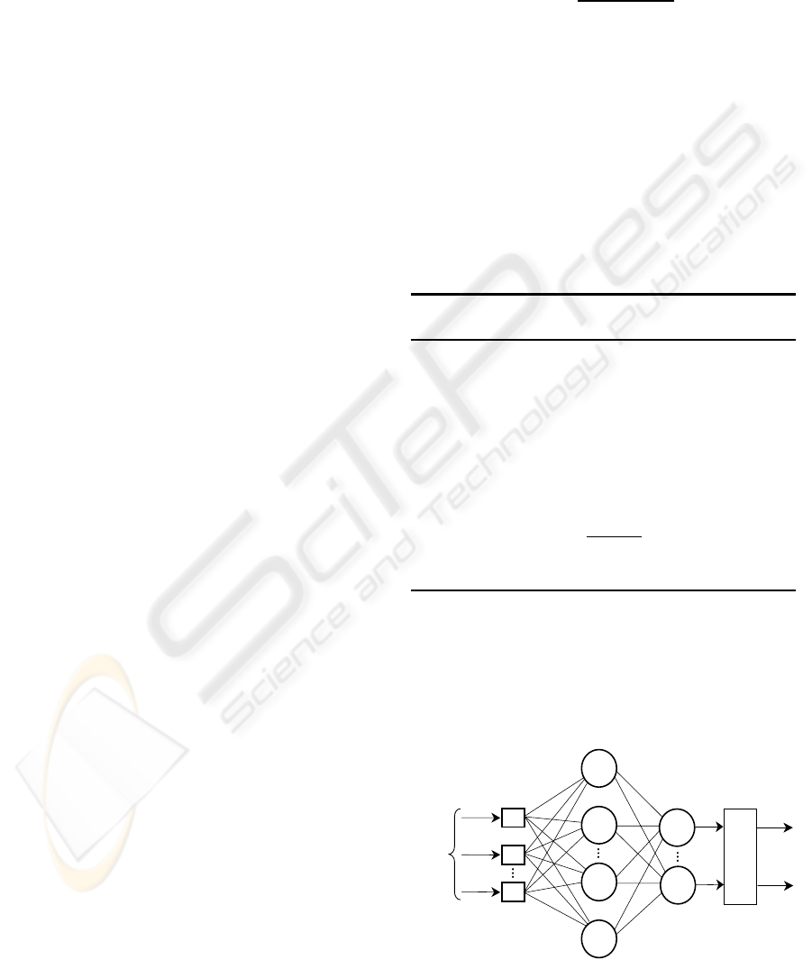
The algorithm is designed to work on-line. The
function approximator adopted to define our policy
is an artificial neural network (ANN) whose weights
represent the policy parameters to be updated at ev-
ery iteration step (see Fig. 2). As input, the network
receives an observation of the state and, as output,
a soft-max distribution evaluates each possible fu-
ture state exponentiating the real-valuedANN outputs
{o
1
, ...,o
n
}, being n the number of neurons of the out-
put layer (Aberdeen, 2003). After applying the soft-
max function, the outputs of the neural network give
a weighting ξ
j
∈ (0, 1) to each of the possible control
actions. The probability of the ith control action is
then given by:
Pr
i
=
exp(o
i
)
∑
n
a=1
exp(o
a
)
(1)
where n is the number of neurons at the output layer.
Actions have been labeled with the associated control
action and chosen at random from this probability dis-
tribution, driving the learner to a new state with its
associated reward.
Once the action has been selected, the error at
the output layer is used to compute the local gradi-
ents of the rest of the network. The whole expres-
sion is implemented similarly to error back propaga-
tion (Haykin, 1999). The old network parameters are
updated following expression 3.(e) of Algorithm 1:
Algorithm 1: Baxter and Bartlett’s OLPOMDP
algorithm.
1. Initialize:
T > 0
Initial parameter values θ
0
∈ R
K
Initial state i
0
2. Set z
0
= 0 (z
0
∈ R
K
)
3. for t = 0 to T do:
(a) Observe state y
t
(b) Generate control action u
t
according to current
policy µ(θ,y
t
)
(c) Observe the reward obtained r(i
t+1
)
(d) Set z
t+1
= βz
t
+
∇µ
u
t
(θ,y
t
)
µ
u
t
(θ,y
t
)
(e) Set θ
t+1
= θ
t
+ α
t
r(i
t+1
)z
t+1
4. end f or
θ
t+1
= θ
t
+ αr(i
t+1
)z
t+1
(2)
The vector of parameters θ
t
represents the network
S
tate
I
nput
Soft-Max
o
1
o
n
1
ξ
n
ξ
Figure 2: Schema of the ANN architecture adopted.
LEARNING BY EXAMPLE - Reinforcement Learning Techniques for Real Autonomous Underwater Cable Tracking
63
weights to be updated, r(i
t+1
) is the reward given to
the learner at every time step, z
t+1
describes the es-
timated gradients mentioned before and, at last, we
have α as the learning rate of the algorithm.
3 CASE TO STUDY: CABLE
TRACKING
This section is going to describe the different ele-
ments that take place into our problem: first, a brief
description of the underwater robot ICTINEU
AUV
and its model used in simulation is given. The sec-
tion will also present the problem of underwater ca-
ble tracking and, finally, a description of the neural-
network controller designed for both, the simulation
and the real phases is detailed.
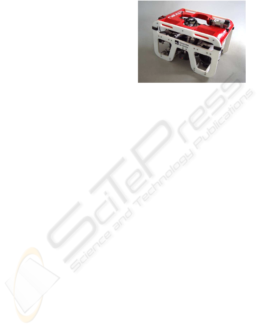
3.1 ICTINEU
AUV
The underwater vehicle ICTINEU
AUV
was originally
designed to compete in the SAUC-E competition that
took place in London during the summer of 2006
(Ribas et al., 2007). Since then, the robot has been
used as a research platform for different underwa-
ter inspection projects which include dams, harbors,
shallow waters and cable/pipeline inspection.
The main design principle of ICTINEU
AUV
was
to adopt a cheap structure simple to maintain and up-
grade. For these reasons, the robot has been designed
as an open frame vehicle. With a weight of 52 Kg,
the robot has a complete sensor suite including an
imaging sonar, a DVL, a compass, a pressure gauge,
a temperature sensor, a DGPS unit and two cameras:
a color one facing forward direction and a B/W cam-
era with downward orientation. Hardware and batter-
ies are enclosed into two cylindrical hulls designed to
withstand pressures of 11 atmospheres. The weight
is mainly located at the bottom of the vehicle, ensur-
ing the stability in both pitch and roll degrees of free-
dom. Its five thrusters will allow ICTINEU
AUV
to be
operated in the remaining degrees of freedom (surge,
sway, heave and yaw) achieving maximum speeds of
3 knots (see Fig. 3).
The mathematical model of ICTINEU
AUV
used
during the simulated learning phase has been obtained
by means of parameter identification methods (Ridao
et al., 2004). The whole model has been uncoupled
and reduced to emulate a robot with only two degrees
of freedom (DOF), X movement and rotation respect
Z axis.
Figure 3: The autonomous underwater vehicle
ICTINEU
AUV
.
3.2 The Cable Tracking Vision System
The downward-looking B/W camera installed on
ICTINEU
AUV
will be used for the vision algorithm
to track the cable. It provides a large underwater field
of view (about 57
◦
in width by 43
◦
in height). This
kind of sensor will not provide us with absolute lo-
calization information but will give us relative data
about position and orientation of the cable respect to
our vehicle: if we are too close/far or if we should
move to the left/right in order to center the object in
our image. The vision-based algorithm used to locate
the cable was first proposed in (Ortiz et al., 2002) and
later improved in (Antich and Ortiz, 2003). It exploits
the fact that artificial objects present in natural envi-
ronments usually have distinguishing features; in the
case of the cable, given its rigidity and shape, strong
alignments can be expected near its sides. The algo-
rithm will evaluate the polar coordinates ρ and Θ of
the straight line corresponding to the detected cable in
the image plane (see Fig. 4).
Once the cable has been located and the polar co-
ordinates of the corresponding line obtained, as the
cable is not a thin line but a large rectangle, we will
also compute the cartesian coordinates (x
g
,y
g
) (see
Fig. 4) of the object’s centroid with respect to the im-
age plane by means of (3).
ρ = xcos(Θ) + ysin(Θ) (3)
where x and y correspond to the position of any point
of the line in the image plane. The computed parame-
ters Θ, x
g
and y
g
together with its derivatives will con-
form the observed state input of the neural-network
controller. For the simulated phase, a downward-
looking camera model has been used to emulate the
vision system of the vehicle.
ICINCO 2008 - International Conference on Informatics in Control, Automation and Robotics
64
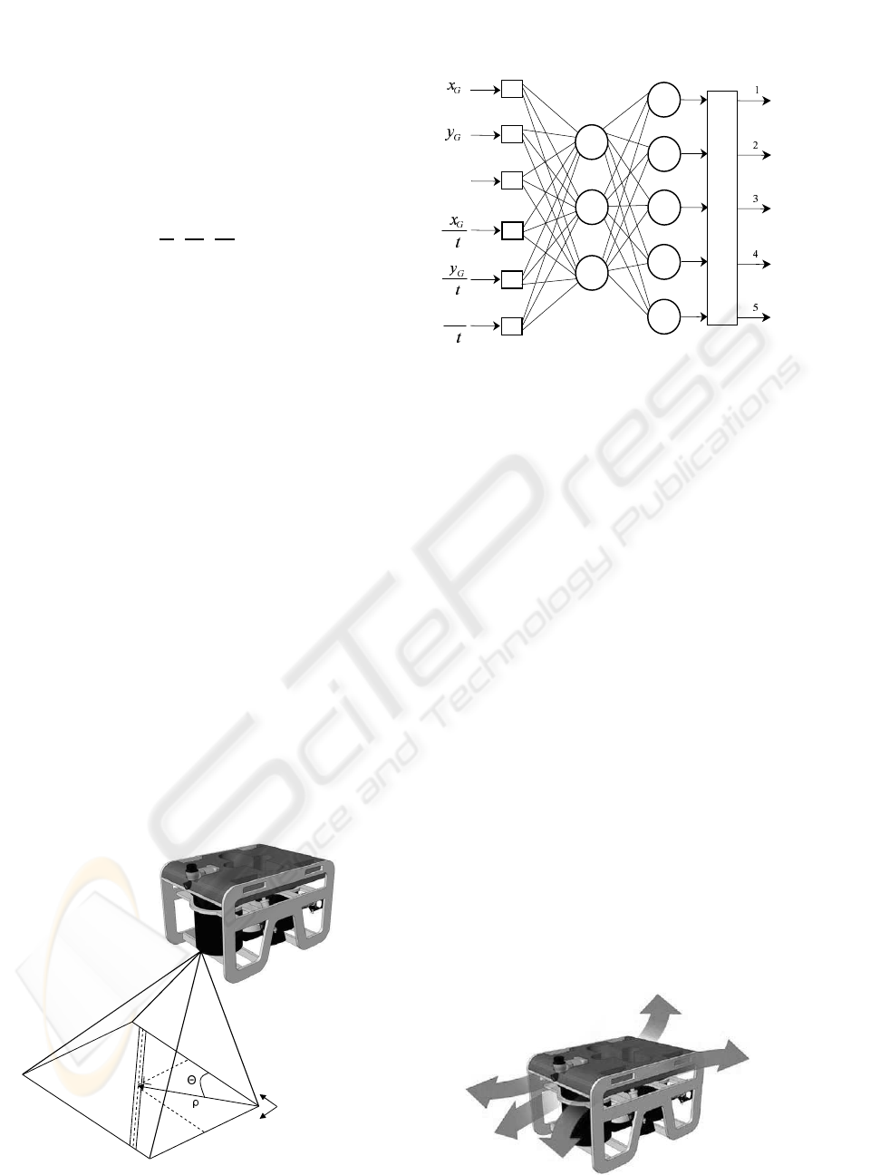
3.3 The Neural-network Controller
A one-hidden-layer neural-network with 6 input
nodes, 3 hidden nodes and 5 output nodes was used
to generate a stochastic policy. As can be seen in
Fig. 5 the inputs to the network correspond to the
normalized state vector computed in the previous
section s = {θ, x
g
, y
g
,
δθ
δt
,
δx
g
δt
,
δy
g
δt
}. Each hidden
and output layer has the usual additional bias term.
The activation function used for the neurons of
the hidden layer is the hyperbolic tangent type,
while the output layer nodes are linear. The five
output neurons represent the possible five con-
trol actions (see Fig. 6). The discrete action set
A = {a
1
, a
2
, a
3
, a
4
, a
5
} has been considered where
A
1
= (Surge,Yaw),A
2
= (Surge, −Yaw),A
3
=
(−Surge,Yaw),A
4
= (−Surge, −Yaw),A
5
=
(Surge, 0). Each action corresponds to a combi-
nation of a constant scalar value of Surge force (X
movement) and Yaw force (rotation respect Z axis).
As explained in Section 2.1, the outputs have been
exponentiated and normalized to produce a probabil-
ity distribution. Control actions are selected at ran-
dom from this distribution.
4 RESULTS
4.1 1rst Phase: Simulated Learning
The model of the underwater robot ICTINEU
AUV
navigates a two dimensional world at 1 meter height
above the seafloor. The simulated cable is placed at
the bottom in a fixed circular position. The controller
X
Y
x
g
f
i
e
l
d
of
v
i
e
w
camera
coordinat
e
frame
yg
Figure 4: Coordinates of the target cable with respect
ICTINEU
AUV
.
Soft-Max
o
1
o
2
ξ
ξ
o
3
o
4
ξ
ξ
Θ
o
5
ξ
∂
∂
∂
∂
∂Θ
∂
Figure 5: The ANN used by the controller.
has been trained in an episodic task. An episode ends
either every 15 seconds (150 iterations) or when the
robot misses the cable in the image plane, whatever
comes first. When the episode ends, the robotposition
is reset to a random position and orientation around
the cable’s location, assuring any location of the ca-
ble within the image plane at the beginning of each
episode. According to the values of the state param-
eters {θ, x
g
, y
g
}, a scalar immediate reward is given
each iteration step. Three values were used: -10, -1
and 0. In order to maintain the cable centered in the
image plane, the positive reward r = 0 is given when
the position of the centroid (x
g
, y
g
) is around the cen-
ter of the image (x
g
± 0.15, y
g
± 0.15) and the angle
θ is close to 90
◦
(90
◦
± 15
◦
), a r = −1 is given in
any other location within the image plane. The re-
ward value of -10 is given when the vehicles misses
the target and the episode ends.
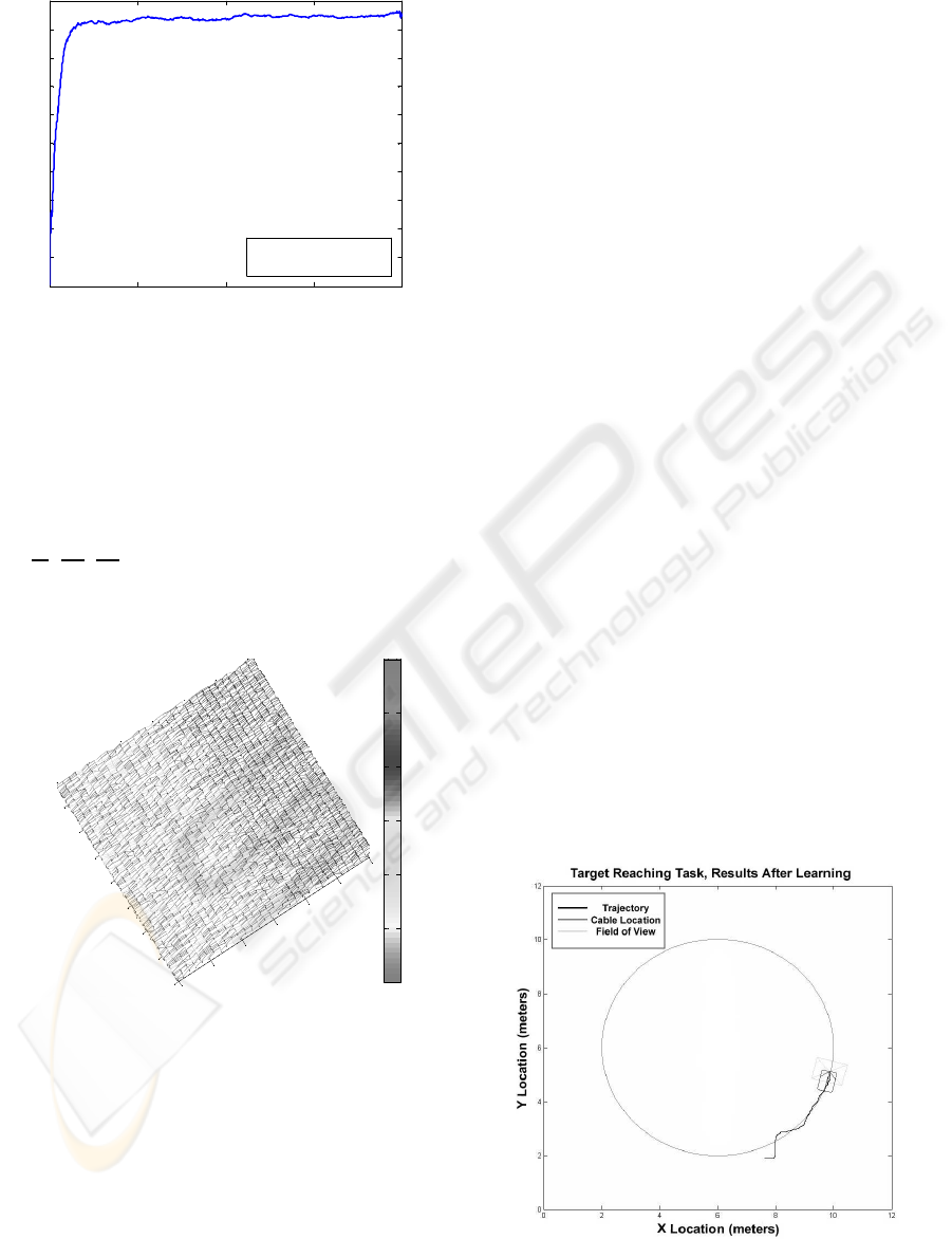
The number of episodes to be done has been set to
2.000. For every episode, the total amount of reward
perceived is calculated. Figure 7 represents the per-
formance of the neural-network robot controller as a
function of the number of episodes when trained us-
ing Baxter and Bartlett’s algorithm on the controller
detailed in Section 3.3. The experiment has been re-
peated in 100 independent runs, and the results here
presented are a mean over these runs. The learning
Figure 6: ICTINEU
AUV
discrete action set.
LEARNING BY EXAMPLE - Reinforcement Learning Techniques for Real Autonomous Underwater Cable Tracking
65
0 500 1000 1500 2000
-200
-180
-160
-140
-120
-100
-80
-60
-40
-20
0
Number of Trials
Mean Total R per Trial
Total R per Trial (mean of 100 rep.)
learning rate 0.001
discount factor 0.98
Figure 7: Performance of the neural-network robot con-
troller as a function of the number of episodes. Performance
estimates were generated by simulating 2.000 episodes.
Process repeated in 100 independent runs. The results are a
mean of these runs. Fixed α = 0.001, and β = 0.98.
rate was set to α = 0.001 and the discount factor β =
0.98. In Figure 8 we can observe a state/action map-
ping of a trained controller, y
g
and the state deriva-
tives
δθ
δt
,
δx
g
δt
,
δy
g
δt
have been fixed in order to represent
a comprehensive graph. Figure 9 represents the tra-
jectory of a trained robot controller.
0
50
100
150
200
250
300
350
-1.5
-1
-0.5
0
0.5
1
1.5
Theta angle (Radiants)
State-Action Mapping Representation, Centroid Y and derivatives fixed
Centroid X Position (Pixels)
1
1.5
2
2.5
3
3.5
4
Figure 8: Centroid X - Theta mapping of a trained robot
controller. The rest of the state variables have been fixed.
Colorbar on the right represents the actions taken.
4.2 2nd Phase: Learned Policy Transfer.
Real Test
Once the learning process is considered to be finished,
the weights of the trained ANN representing the pol-
icy are transferred to ICTINEU
AUV
and its perfor-
mance tested in a real environment. The robot’s con-
troller is the same one used in simulation. The experi-
mental setup can be seen in Fig. 10 where the detected
cable is shown while the vehicle performs a test inside
the pool. Fig. 11 represents real trajectories of the θ
angle of the image plane while the vehicle performs
different trials to center the cable in the image.
5 CONCLUSIONS AND FUTURE
WORK
This paper proposes a field application of a high-
level Reinforcement Learning (RL) control system
for solving the action selection problem of an au-
tonomous robot in cable tracking task. The learn-
ing system is characterized by using a direct policy
search algorithm for robot control based on Baxter
and Bartlett’s direct-gradient algorithm. The policy
is represented by a neural network whose weights are
the policy parameters. In order to speed up the pro-
cess, the learning phase has been carried out in a sim-
ulated environment and then transferred and tested
successfully on the real robot ICTINEU
AUV
.
Results of this work show a good performance of
the learned policy. Convergence times of the simu-
lation process were not too long if we take into ac-
count the reduced dimensions of the ANN used in the
simulation. Although it is not a hard task to learn in
simulation, continue the learning autonomously in a
real situation represents a challenge due to the nature
of underwater environments. Future steps are focused
on improving the initial policy by means of on-line
learning processes and comparing the results obtained
with human pilots tracking trajectories.
Figure 9: Behavior of a trained robot controller, results of
the simulated cable tracking task after learning period is
completed.
ICINCO 2008 - International Conference on Informatics in Control, Automation and Robotics
66
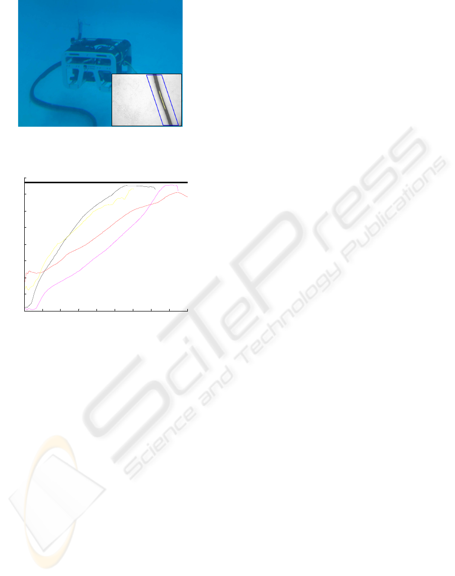
Figure 10: ICTINEU
AUV
in the test pool. Small bottom-
right image: Detected cable.
0 20 40 60 80 100 120 140 160 18
0
0.8
0.9
1
1.1
1.2
1.3
1.4
1.5
1.6
Number of Iterations
Theta angle (Radiants)
Real Variation of the Theta angle while attempting to center the cable
Figure 11: Real measured trajectories of the θ angle of the
image plane while attempting to center the cable.
ACKNOWLEDGEMENTS
This work has been financed by the Spanish Govern-
ment Comission MCYT, project number DPI2005-
09001-C03-01, also partially funded by the MO-
MARNET EU project MRTN-CT-2004-505026 and
the European Research Training Network on Key
Technologies for Intervention AutonomousUnderwa-
ter Vehicles FREESUBNET, contract number MRTN-
CT-2006-036186.
REFERENCES
Aberdeen, D. A. (2003). Policy-Gradient Algorithms
for Partially Observable Markov Decision Processes.
PhD thesis, Australian National University.
Anderson, C. (2000). Approximating a policy can be easier
than approximating a value function. Computer sci-
ence technical report, University of Colorado State.
Antich, J. and Ortiz, A. (2003). Underwater cable track-
ing by visual feedback. In First Iberian Conference
on Pattern recognition and Image Analysis (IbPRIA,
LNCS 2652), Port d’Andratx, Spain.
Atkenson, C., Moore, A., and Schaal, S. (1997). Lo-
cally weighted learning. Artificial Intelligence Re-
view, 11:11–73.
Bagnell, J. and Schneider, J. (2001). Autonomous he-
licopter control using reinforcement learning policy
search methods. In Proceedings of the IEEE Interna-
tional Conference on Robotics and Automation, Ko-
rea.
Baxter, J. and Bartlett, P. (1999). Direct gradient-based rein-
forcement learning: I. gradient estimation algorithms.
Technical report, Australian National University.
El-Fakdi, A., Carreras, M., and Ridao, P. (2006). Towards
direct policy search reinforcement learning for robot
control. In IEEE/RSJ International Conference on In-
telligent Robots and Systems.
Hammer, B., Singh, S., and Scherer, S. (2006). Learning
obstacle avoidance parameters from operator behav-
ior. Journal of Field Robotics, Special Issue on Ma-
chine Learning Based Robotics in Unstructured Envi-
ronments, 23 (11/12).
Haykin, S. (1999). Neural Networks, a comprehensive foun-
dation. Prentice Hall, 2nd ed. edition.
Kohl, N. and Stone, P. (2004). Policy gradient reinforce-
ment learning for fast quadrupedal locomotion. In
IEEE International Conference on Robotics and Au-
tomation (ICRA).
Konda, V. and Tsitsiklis, J. (2003). On actor-critic algo-
rithms. SIAM Journal on Control and Optimization,
42, number 4:1143–1166.
Lin, L. (1992). Self-improving reactive agents based on re-
inforcement learning, planning and teaching. Machine
Learning, 8(3/4):293–321.
Marbach, P. and Tsitsiklis, J. N. (2000). Gradient-based op-
timization of Markov reward processes: Practical vari-
ants. Technical report, Center for Communications
Systems Research, University of Cambridge.
Matsubara, T., Morimoto, J., Nakanishi, J., Sato, M., and
Doya, K. (2005). Learning sensory feedback to CPG
with policy gradient for biped locomotion. In Pro-
ceedings of the International Conference on Robotics
and Automation ICRA, Barcelona, Spain.
Meuleau, N., Peshkin, L., and Kim, K. (2001). Explo-
ration in gradient based reinforcement learning. Tech-
nical report, Massachusetts Institute of Technology,
AI Memo 2001-003.
Ortiz, A., Simo, M., and Oliver, G. (2002). A vision system
for an underwater cable tracker. International Journal
of Machine Vision and Applications, 13 (3):129–140.
Ribas, D., Palomeras, N., Ridao, P., Carreras, M., and Her-
nandez, E. (2007). Ictineu auv wins the first sauc-
e competition. In IEEE International Conference on
Robotics and Automation.
Ridao, P., Tiano, A., El-Fakdi, A., Carreras, M., and Zirilli,
A. (2004). On the identification of non-linear models
of unmanned underwater vehicles. Control Engineer-
ing Practice, 12:1483–1499.
LEARNING BY EXAMPLE - Reinforcement Learning Techniques for Real Autonomous Underwater Cable Tracking
67

Rosenstein, M. and Barto, A. (2001). Robot weightlifting
by direct policy search. In Proceedings of the Interna-
tional Joint Conference on Artificial Intelligence.
Smart, W. (2002). Making Reinforcement Learning Work
on Real Robots. PhD thesis, Department of Computer
Science at Brown University, Rhode Island.
Sutton, R. and Barto, A. (1998). Reinforcement Learning,
an introduction. MIT Press.
Sutton, R., McAllester, D., Singh, S., and Mansour, Y.
(2000). Policy gradient methods for reinforcement
learning with function approximation. Advances in
Neural Information Processing Systems, 12:1057–
1063.
Tedrake, R., Zhang, T. W., and Seung, H. S. (2004).
Stochastic policy gradient reinforcement learning on
a simple 3D biped. In IEEE/RSJ International Con-
ference on Intelligent Robots and Systems IROS’04,
Sendai, Japan.
ICINCO 2008 - International Conference on Informatics in Control, Automation and Robotics
68
