
ROBOT GOES BACK HOME DESPITE ALL THE PEOPLE
Paloma de la Puente, Diego Rodriguez-Losada, Luis Pedraza and Fernando Matia
DISAM - Universidad Politecnica de Madrid, Jose Gutierrez Abascal 2, Madrid, Spain
Keywords:
Mobile Robots Navigation, Localization and Mapping, Reactive Control, Dynamic Points.
Abstract:
We have developed a navigation system for a mobile robot that enables it to autonomously return to a start
point after completing a route. It works efficiently even in complex, low structured and populated indoor
environments. A point-based map of the environment is built as the robot explores new areas; it is employed
for localization and obstacle avoidance. Points corresponding to dynamical objects are removed from the map
so that they do not affect navigation in a wrong way. The algorithms and results we deem more relevant are
explained in the paper.
1 INTRODUCTION
Autonomous navigation around indoor environments
is a difficult task for a mobile robot to achieve, es-
pecially if there are people passing by frequently. A
good start point is presented in (Borenstein et al.,
1996) by breaking down the general problem of
robot navigation into three questions:”Where am I?”,
”Where am I going?”, ”How should I get there?”. So,
the first (and main) problem encountered when deal-
ing with this issue is the necessity of knowing where
the robot is at every moment.As the robot moves, er-
rors in odometry information increase significantly
hence making it essential that these data be corrected.
Different probabilistic methods for performing this
correction using measurements received from stereo-
ceptive sensors (such as laser range-finders or sonars)
have thus far been developed, being those capable of
building a map at the same time for proper representa-
tion of the environment the most effective and popular
ones.
As for the second question, the goal to be reached
is often defined by the user. It may be given by higher
level tasks depending on the particular application.
The last question is challenging as well. A first
step is motion control, which is better addressed by
means of a closed-loop controller using position feed-
back (Siegwart and Nourbakhsh, 2004). With a reg-
ulator of this kind, path planning comes to comput-
ing a sequence of passing points leading to the tar-
get. Once a nominal trajectory has been obtained,
safe navigation requires reactive control, for the robot
should be able to change its behavior if a situation
that endangers its mission appears. Regarding this,
several strategies have been used in the literature to
face obstacle avoidance. Some of the proposed solu-
tions (Feiten et al., 1994), (Yang and Li, 2002) consist
of sending special drive and steer velocity commands
when an obstacle is detected. The latter and other
authors do so through fuzzy control. An interesting
and generic approach is an iterative algorithm found
in (Lamiraux et al., 2004) for real time deformation
of previously collision free paths when operating with
nonholonomic robots.
Dynamic objects in the environment bring about
further difficulties in map building and reactive con-
trol. If the problem is simplified and observed fea-
tures are represented as permanent in the map, it is
still useful for localization purposes but there will be
discrepancies with reality. It also increases the map’s
size unnecessarily and may result in the robot avoid-
ing obstacles which are no longer there. (R.Siegwart
et al., 2002) tackle this issue applying the EM algo-
rithm and making use of an a priori map of the en-
vironment. They also address other aspects of robot
navigation in populated exhibitions, remarking the
importance of introducing novel combinations and
adaptations of different preexisting approaches. (Hh-
nel et al., 2003) developed a statistical method to
identify measurements corresponding to dynamic ob-
jects and perform localization and building of occu-
pancy grid maps, all in the context of the EM algo-
rithm.
In this paper we present a system which allows
208
de la Puente P., Rodriguez-Losada D., Pedraza L. and Matia F. (2008).
ROBOT GOES BACK HOME DESPITE ALL THE PEOPLE.
In Proceedings of the Fifth International Conference on Informatics in Control, Automation and Robotics - RA, pages 208-213
DOI: 10.5220/0001491502080213
Copyright
c
SciTePress

the robot to build a point-based map of its static sur-
roundings while being teleoperated from somewhere;
this map is afterwards used by the robot to localize it-
self and make its way back to its original pose, avoid-
ing any obstacles which may be near the initial path.
Experiments in highly crowded and cluttered environ-
ments have been carried out successfully.
This work is to be used in an ambitious project
concerning the autonomous setup of an interactive
robot at museums and trade fairs. The robot’s name
is Urbano and it already counts on a robust local-
ization system based upon geometrical features over
SLAM-EKF that originates 2D precise maps in real
time (Rodr
´
ıguez-Losada, 2004). Here we expose an
efficient less complex model with the specific demon-
strator of the returning home utility. This work has
been partially founded by DPI-2004-07907-C02-01.
The paper is organized as follows. Section 2 in-
cludes a description of the algorithms corresponding
to localization and mapping. In Section 3 we present
the movement and reactive control implemented al-
gorithms. Section 4 accounts for experimental results
we have obtained. Finally, Section 5 contains our con-
clusions and future working lines.
2 LOCALIZATION AND
MAPPING
2.1 Localization and Map Building
The solution adopted for this problem is a Maxi-
mum Incremental Probability algorithm whose foun-
dation is the Extended Kalman Filter(EKF). The sys-
tem elaborates and continually updates a map built
from the observations acquired from the laser mea-
surements.
The state vector used is defined as the robot’s
global pose, [x
R
,y
R
,θ
R
]
T
, whereas the odometry mea-
surements (incremental, so referred to the robot’s lo-
cal coordinate system) represent the system inputs,
~u = [u
x
,u
y
,θ
u
]
T
. Time subscripts are omitted in the
latter so as to simplify notation; measurements ob-
tained last are always the ones considered. According
to this, the state equation is put as:
~x
R
k
=~x
R
k−1
⊕~u = f (~x
R
k−1
,~u) (1)
where ⊕ represents the composition of relative trans-
formations.Odometry measurements can be modelled
as a gaussian variable, ~u
k
∼ N(
ˆ
~u
k
,Q).
2.1.1 Predictor Equations
Applying the definition of the ⊕ operator, the pre-
dicted state, ˜x
R
k
, will be given by:
˜x
R
k
˜y
R
k
˜
θ
R
k
=
ˆx
R
k−1
+ u
x
cos
ˆ
θ
R
k−1
− u
y
sin
ˆ
θ
R
k−1
ˆy
R
k−1
+ u
x
sin
ˆ
θ
R
k−1
+ u
y
cos
ˆ
θ
R
k−1
ˆ
θ
R
k−1
+ θ
u
(2)
And the state’s covariance prediction,
˜
P
k
, is computed
from:
˜
P
k
= F
x
ˆ
P
k−1
F
T
x
+ F
u
QF
T
u
(3)
being F
x
=
δ f
δ~x
|
˜
~x
R
k
, F
u
=
δ f
δ~u
|
˜
~x
R
k
(we use the best state
estimation obtained up to now)
The algorithm is initiated with ˆx
0
= 0,
ˆ
P
0
= 0.
2.1.2 Corrector Equations and Data Association
Ideally, each observation ~o
i
= [o
ix
,o
iy
]
T
(or laser mea-
surement received) is implicitly related to the pre-
vious estimation of the state by means of compo-
sition with it and comparison to the corresponding
~
l
j
= [x
l j
,y
l j
]
T
point in the map. The resultant expres-
sion is known as the innovation of observation i:
~
h
i j
= ~x
R
⊕~o
i
−
~
l
j
= h(~x
R
,~o
i
,
~
l
j
) =
~
0 (4)
which combined with ⊕ definition is the same as:
~
h
i j
=
−x
l j
+ ˜x
R
+ o
ix
cos
˜
θ
R
− o
iy
sin
˜
θ
R
−y
l j
+ ˜y
R
+ o
ix
sin
˜
θ
R
+ o
iy
cos
˜
θ
R
=
~
0 (5)
If we denote H
x
i j
k
=
δ
~
h
i j
δ~x
|
˜
~x
R
k
,~o
i
, H
z
i j
k
=
δ
~
h
i j
δ~o
i
|
˜
~x
k
,~o
i
for
every iteration k, the covariance of each innovation is
given by:
S
i j
k
= H
x
i j
k
˜
P
k
H
T
x
i j
k
+ H
z
i j
k
RH
T
z
i j
k
(6)
where R is the covariance of laser measurements.
We have followed the Nearest Neighbor strategy
to pair each observation with its correspondent map
point. Computation of the Mahalanobis distance for
innovation h
i j
k
once we have got its covariance matrix
S
k
will let us select that map point which minimizes
such distance. If Mahalanobis test is passed for that
association, then it is taken into account at the correc-
tion step; otherwise it will be added as a new point of
the map vector. Among all the h
i j
,H
x
i j
and H
zi j
matri-
ces obtained for an observation at a certain iteration,
only those corresponding to the map point, if any, as-
sociated to it will be kept to correct the estimation.
They will be denoted h
i
min
,H
xi
min
,H
zi
min
. As more as-
sociations are made, there are more measurements to
ROBOT GOES BACK HOME DESPITE ALL THE PEOPLE
209

be used. This is contemplated by filling other matri-
ces containing joint information from all of them:
~
h = [h
1
min
,...,h
t
min
]
T
(7)
H
x
= [H
x1
min
,...,H
xt
min
]
T
(8)
H
z
=
H
z1
min
.
.
.
h
t
min
(9)
where t is the total number of associations. Now we
get the global S matrix and the Kalman gain from
S = H
x
˜
PH
T
x
+ H
z
RH
T
z
(10)
K =
˜
PH
T
x
S
−1
(11)
The corrected values are updated from this informa-
tion and the prediction values obtained from 2 and 3:
ˆ
~x =
˜
~x − Kh; (12)
ˆ
P = (I − KH
x
)
˜
P (13)
2.2 Removal of Dynamic Points
The algorithm presented above incorporates to the
map every observed point which cannot be associated
to a pre-existing one. If we stick to it, points cor-
responding to a dynamic object detected at a given
moment are included in the map when they are first
seen (just as any other object is) and nothing is done
to avoid them being there forever. Here we propose
a method that removes map points far from being ob-
served at a given moment, before the correction and
update of the map take place.
Firstly, an evolvent polygon of the laser measure-
ments is constructed in a recursive way. The general
procedure is summarized in the following lines:
• A segment from the first measurement to the last
is taken.
• The furthest observation from that segment is
sought among the others.
• If the separation between the segment and that ob-
servation is high enough, the process is repeated
between the first observation and the one selected
and then between this observation and the last
one.
• When for one segment there is no observation at
a greater distance than a threshold, its limits are
stored in a vector containing the polygon vertices.
Some other simplifications are made in order not to
generate too many vertices. Map points that remain
quite inside the polygon cannot correspond to cur-
rently observed objects because if so, they would ei-
ther have been included as polygon vertices or they
would be very close to them (due to the threshold and
the simplifications mentioned above).
β
α
4
α
5
β
α
2
α
3
α
6
α
1
Figure 1: Angles to be measured for seeing if a point is
inside an unconvex polygon.
To find out whether a map point is inside the poly-
gon, we compute a series of angles (α
1
...α
v
in figure
1) as soon as the vertices extraction is over. Then,
for every point in the map which is not too near the
polygon’s border we determine its coordinates in the
laser reference system and then compute the value of
the β angle represented in the same figure. Selecting
those alphas β lies in between (α
1
and α
2
in the fig-
ure’s case) we obtain the corresponding vertices and
use their distance to the robot to establish if that map
point should be erased. We use a conservative crite-
rion that leaves outside the map only those points at a
smaller distance than the closest of both vertices. This
prevents any map points being removed incorrectly.
The computational cost of creating the polygon
and finding the values of the needed angles is upper
bounded, since the number of observations provided
by the laser is constant. Notice that only one angle
has to be computed for each point in the map, which
makes it a not very cumbersome algorithm.
3 MOTION CONTROL
3.1 Motion Controller
To get the robot moving from one point to another
we have employed gain scheduling, implementing a
controller in agreement to the divide and conquer ap-
proach. The error is a linear combination of three
angles. In first place is the difference between the
present orientation of the robot and the one it should
ICINCO 2008 - International Conference on Informatics in Control, Automation and Robotics
210
have to look straight ahead to the next goal. The sec-
ond angle is that one the robot should turn to have the
same global orientation as the current trajectory seg-
ment it is at. The third angle is similar to the second
although in this case it is the next trajectory segment
that is considered. Weights of 0.3, 0.2 and 0.5 have
been used to produce smooth anticipative movement
following a given trajectory. We define several inter-
vals for that global error and vary a constant value of
drive velocity and the gain of a proportional controller
for the steer velocity within each of them.
In the experiments described here, the given tra-
jectory is obtained by saving the robot’s pose every
time it moves a constant distance.
Nominalpath
Collisionpath
Correctedpath
Goal
Ob t l
Start
Ob
s
t
ac
l
e
Start
Robot
Figure 2: Possible paths if the robot is not near the defined
trajectory.
If the robot were to be quite separated from the
defined trajectory, this controller would take it to the
goal not across the nominal path but across one in
which there might be an obstacle(figure 2).
The corrected path is obtained by forcing the robot
to approach the nominal path before heading for the
target. For this purpose we have included control laws
that regulate angles δ
1
or δ
2
in figure 3 depending on
which side of the path the robot is at. We use an-
gles in [−π,π] along all our work, which is what the
ForceInRange function has been defined for. These
laws are employed instead of the initial ones only
when the robot is far enough from the defined path.
When the robot is told to go back, it turns 180 at
first and then come into action the rules that have just
been commented. At a certain distance from home,
the robot begins to slow down until it reaches its fi-
nal pose. Then it turns to adopt the orientation it had
when it abandoned home.
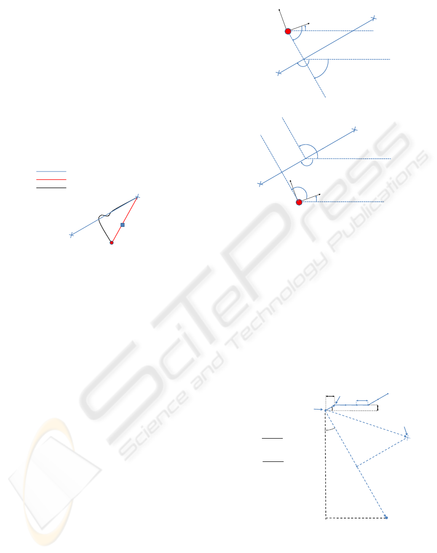
3.2 Path Deformation
To get a trajectory free of obstacles we displace the
points of the nominal trajectory which are affected by
objects detected in the environment.To begin with, we
make sure that consecutive points in the initial trajec-
tory are at a short enough distance, let it be 0.1m.For
each point i we follow the same steps. At first, a point
Goal
y
R
x
R
δ
θ
δ
1
an
g
1
ang1+ PI/2
Start
g
ang1+
PI/2
δ
1
= ang1+PI/2‐ θ
Goal
ForceInRange(ang1‐ PI/2)
Start
y
R
ang1
δ
x
R
θ
δ
2
δ
2
=
ForceInRan
g
e
(
an
g
1‐ PI
/
2
)
‐
θ
2
g
(g
/)
Figure 3: Angles through which control is executed.
p is defined on the normal to the segment joining that
point of the trajectory and the next one so that it is 1m
away from the former. The vector going from point i
to point p will be referred to as v
1
. We define a vector
v
2
with origin at the considered trajectory point and
end at the subsequent obstacles detected. The orthog-
onal projection of this vector v
2
onto v
1
determines
point p
2
. Its distance to the trajectory point i is d,
which may be positive or negative if the obstacle is at
one side or another of the trajectory.
0.1
x
1
‐x
0
(x
1
,y
1
)
α
y
1
‐y
0
(x
0
,y
0
)
v
bl
α
)
(
10
sin
01
y
y
y
y
−
α
v
2
o
b
stac
l
e
)
(
10
1.0
sin
01
y
y
y
y
−
=
=
α
d
d
)(10
1.0
cos 01
01
xx
x
x
−=
−
=
α
d
1
p
2
|
v
|
= 1
x
p
=x
0
+sinα=x
0
+10(y
1
‐ y
0
)
y
p
=
y
0
–
cos
α
=
y
0
‐
10(x
1
‐
x
0
)
p (
x
y
)
|
v
1
|
=
1
y
p
y
0
cos
α
y
0
10(x
1
x
0
)
v
1
p
=
(
x
p
,
y
p
)
Figure 4: Definition of point p and other magnitudes for the
trajectory point i = 0.
The distance from p
2
to the obstacle will be called
d
1
. All these magnitudes are represented in figure
4.Only those objects resulting in a small enough value
of d
1
take part in the deformation relative to that
ROBOT GOES BACK HOME DESPITE ALL THE PEOPLE
211
i+1
i
i’
Figure 5: Displacement applied to each point of the nominal
trajectory.
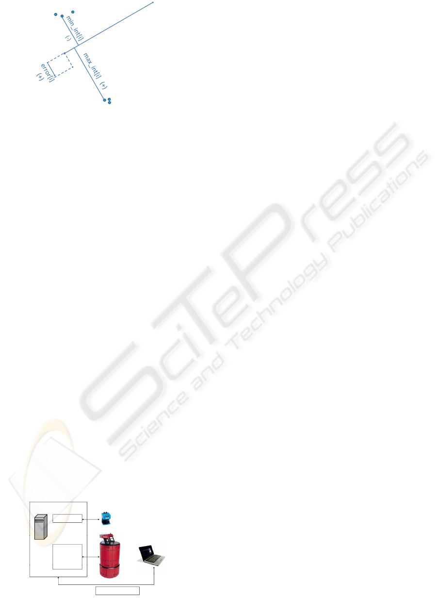
path point. Correcting d by considering the influ-
ence of the robot radius and afterwards obtaining its
minimum and maximum values, an area of permitted
movement can be determined. We will call these two
distances min_int[i] and max_int[i], respectively.
They are initialized with the maximum displace-
ment allowed, for the case of no presence of obstacles
and other similar situations. Their mean will be the
displacement,error [i], to apply to that path point in
order to leave it at an intermediate distance between
the limits found for each of both sides (see figure 5).
To generate a smoother deformation we use the aver-
age of that error value and the previous and next ones:
error2[i] = (error[i − 1] + error[i] + error[i + 1])/3
4 EXPERIMENTS AND RESULTS
The system has been tested in different environments,
using simulators (one we have developed ourselves
and also MobileSim, by Activemedia Robotics) and
real robot data from text files at the beginning, and the
robot Urbano afterwards. Urbano stands on a B21r
platform and has a laser SICK LMS200 mounted on
top. The architecture of the system is the one in fig.
6.
The most significant experiments we have con-
ducted took place at our laboratory, which has very
narrow areas and people often coming to and fro. The
Robot PC
LMS 200
Robot
PC
Serial Port
LMS
200
B21r
Client PC
Mobility
Server
TCP streams
Figure 6: Urbano’s distribution schema.
robot was teleoperated from one end of the laboratory
to the other, finding a lot of visitors while building the
map.When we had brought it to the main entrance, we
told him to return home. Since that moment all of its
behavior is absolutely autonomous. In the way back,
other people were seen and Urbano was able to avoid
them. Some other slight corrections were made in or-
der to follow a path which got apart from close obsta-
cles. One of the maps we obtained is the one in figure
7. The green path is the odometry corresponding to
the teleoperation mode. The pink path is the one rep-
resenting dead-reckoning in the way back. The blue
trajectory is the correction for the first stage of the ex-
periment, while the red one is the correction obtained
when the robot was coming back home. Cyan points
are those which were removed from the map. Most of
them were clearly identified with people’s successive
positions when walking in front of the robot.
Another experiment was performed in the build-
ing where lessons are imparted at a time in which
there were plenty of students coming out from their
classes. The resultant map and the actual environment
are shown in figure 8.
5 CONCLUSIONS
The system presented here has two main components,
one having to do with localization and map building
and one related to control and path deformation.
The implemented localization and mapping algo-
rithm is a Maximum Incremental Probability method
based on the Extended Kalman Filter (EKF). Its main
drawback is the fact that it does not consider the un-
certainty in the map itself, but it allows for a higher
degree of simplicity and has proven an appropriate
behavior on the experimental conditions of a wide va-
riety of tests apart from those exposed in this paper
(using data obtained by several real robots in differ-
ent indoor environments, some of them having large
odometry errors). The elimination of points makes
more realistic and reliable maps which represent the
last structure observed by the robot. If the same map
were used in another experiment, instead of making
the robot build a new one in real time,it would get
adapted to the configuration of the environment at that
moment. This strategy also prevents mistakes in data
association and reduces maps’ size when possible.
The developed control module enables the robot
to achieve a final target without hitting any obstacles.
A high level technique keeps the path to be followed
away from the objects detected by the laser, and the
controller does not let the robot get far from this col-
lision free path. Obstacles at lower height than the
ICINCO 2008 - International Conference on Informatics in Control, Automation and Robotics
212
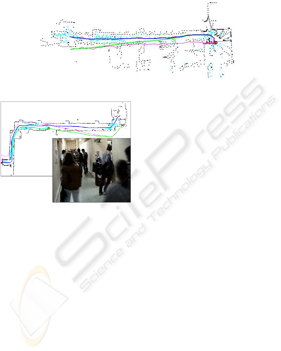
Figure 7: Real time built map of our laboratory.
Figure 8: Real time built map of an area plenty of students.
laser sensor cannot be seen. Consequently, not only
will these obstacles be left out of the map and cause
it to be less accurate but, what is much worse, they
will not be considered in path deformation either. As
a precaution, Urbano has got some ultrasound sensors
at an intermediate height which make the robot stop
if they detect it is about to crash, but it might not be
enough under some circumstances. This caveat gives
rise to one of our next working lines.
6 FUTURE WORK
As previously mentioned, we now orientate our work
towards the integration of knowledge models for the
autonomous setup of an interactive robot at museums
and trade fairs. The reference of this project, called
Robonauta, is:DPI2007-66846-c02-01.
To achieve this important objective, some lines re-
lated to this work and to Urbano’s navigation in gen-
eral are:
• Extension of geometrical models. Employing a
wrist that can precisely position the 2D scanner
in different angles for data acquisition, we aim at
constructing robust algorithms to create 3D maps
which will make the robot’s navigation safer.
• Improvements in control, so that the robot can
move faster and follow its path more accurately.
• Path definition by means of people tracking or by
means of voice commands spoken to the robot.
• Incorporation of new conducts which will enable
the robot to follow a learning process by itself.
REFERENCES
Borenstein, J., Everett, H., and L.Feng (1996). Navigating
Mobile Robots: Systems and Techniques. A.K Peters.
Feiten, W., R.Bauer, and Lawitzky, G. (1994). Robust Ob-
stacle Avoidance in Unknown and Cramped Environ-
ments. In IEEE Int. Conf. Robotics and Automation.
Hhnel, D., R.Triebel, W.Burgard, and S.Thrun (2003). Map
Building with Mobile Robots in Dynamic Environ-
ments. In IEEE Int. Conf. Robotics and Automation.
Lamiraux, F., Bonnafous, D., and O.Lefebvre (2004). Re-
active Path Deformation for Nonholonomic Mobile
Robots. IEEE Transactions on Robotics.
Rodr
´
ıguez-Losada, D. (2004). SLAM Geom
´
etrico en
Tiempo Real para Robots M
´
oviles en Interiores
basado en EKF. PhD thesis, ETSII-Universidad
Politcnica de Madrid.
R.Siegwart, R.Philippsen, and B.Jensen (2002).
http://robotics.epfl.ch.
Siegwart, R. and Nourbakhsh, I. (2004). Introduction to
Autonomous Mobile Robots. MIT Press.
Yang, S. and Li, H. (2002). An Autonomous Mobile Robot
with Fuzzy Obstacle Avoidance Behaviors and a Vi-
sual Landmark Recognition System. In 7
th
ICARCV.
ROBOT GOES BACK HOME DESPITE ALL THE PEOPLE
213
