
SELF CONSTRUCTING NEURAL NETWORK ROBOT
CONTROLLER BASED ON ON-LINE TASK PERFORMANCE
FEEDBACK
Andreas Huemer
a
, Mario Gongora
b
and David Elizondo
b
a
Institute Of Creative Technologies, De Montfort University, Leicester, U.K.
b
Centre for Computational Intelligence, De Montfort University, Leicester, U.K.
Keywords:
Spiking neural network, reinforcement learning, robot controller development.
Abstract:
A novel methodology to create a powerful controller for robots that minimises the design effort is presented.
We show that using the feedback from the robot itself, the system can learn from experience. A method
is presented where the interpretation of the sensory feedback is integrated in the creation of the controller,
which is achieved by growing a spiking neural network system. The feedback is extracted from a performance
measuring function provided at the task definition stage, which takes into consideration the robot actions
without the need for external or manual analysis.
1 INTRODUCTION
Machine intelligence and machine learning tech-
niques have been used extensively in the tuning and
optimisation of robot controllers capable of enabling
the execution of complex tasks. Similarly, given
the vast variety of possible conditions present in the
real world, machine learning has been the subject of
significant research to improve the responses of au-
tonomous robots to a variety of situations. But the
use of these techniques in the actual design of the con-
trollers is still in its early stages. This paper presents a
novel methodology capable of creating a spiking neu-
ral based controller, which is being studied and eval-
uated as part of our research in autonomous robots.
Our method also takes into account the aspect of on-
line learning which is a much more intuitive approach
to real world problems, specifically for the study of
robotics in non-structured environments.
One type of learning system that has been applied
successfully to some control problems is based on
neural networks. One approach to have robots that
are able to adapt to completely new situations could
be to provide a neural network with enough fully con-
nected neurons, and have those connections adapted
with known machine learning methods; this, in prin-
ciple, would provide enough adaptable components
in their control system. Alternatively, as has been
shown by Elizondo et al. (Elizondo et al., 1995), par-
tially connected neural networks are faster to train and
have better generalisation capabilities. Similar effects
have been found considering the number of neurons
(Gómez et al., 2004), where it has been shown that it
is not necessarily better to have more neurons.
In this paper we present a novel method for cre-
ating a neural network based robot controller which
starts with a minimalistic neural network having a
small number of neurons and connections and grow it
until it can fulfil effectively the tasks required by the
robot. The results presented have been evaluated with
a set of experiments where a simulated robot learns to
avoid obstacles while wandering around in a room.
We have created a self constructing controller for
a robot which consists of a spiking neural network
which learns from experience by connecting the neu-
rons, adapting the connections and growing new neu-
rons depending on a feedback process that will cor-
respond to the measurement of a perceived “gratifi-
cation” value of the robot. The measurement of the
“gratification” that the robot perceives can be defined
by an evaluation function that rewards the robot de-
pending on the performance of the task, causing that
the neural network develops itself. This self construc-
tion occurs without the need of any external or hu-
man intervention, creating a purely automated learn-
ing mechanism; the self construction can be guided
326
Huemer A., Gongora M. and Elizondo D. (2008).
SELF CONSTRUCTING NEURAL NETWORK ROBOT CONTROLLER BASED ON ON-LINE TASK PERFORMANCE FEEDBACK.
In Proceedings of the Fifth International Conference on Informatics in Control, Automation and Robotics - ICSO, pages 326-333
DOI: 10.5220/0001495503260333
Copyright
c
SciTePress

as well with runtime feedback from a trainer (either
automated or human operated), representing the vali-
dation of an expert.
Reward based systems have been presented, as in
(Florian, 2005) where a worm that was fed with pos-
itive reward when its mouth was moving towards its
food source and negative reward when its mouth was
moving in the other direction was simulated using a
neural network to control its movements. Depend-
ing on the feedback the connections between the neu-
rons were adapted, which finally took the mouth of
the worm to the food source. A similar method was
used in the experiments of this paper. A reward mea-
surement will be used both for growing new neurons
and for adapting the connections between them.
During the creation of the network we have sep-
arated the neural connections in two parts: artificial
dendrites and axons. These do not only play an im-
portant role with the growth mechanism but in the ba-
sic decision mechanism for the actions.
At this stage of the research we have set some ini-
tial constraints to provide a reliable evaluation of the
novel growth methods. For example recurrent con-
nections and Spike Time Dependent Plasticity have
been excluded, which would both increase the capa-
bilities of the neural network as for example shown by
Gers et al. (Gers et al., 2002) or Izhikevich (Izhike-
vich, 2006). However, they would also increase the
dynamics of the network and hence the effort of eval-
uating it and the certainty of the evaluation at this ini-
tial stage.
The paper is organised in the following way. Sec-
tion 2 explains the principle of the type of connections
used in our neural network. In section 3 the basic
learning mechanisms of the spiking neural network
are described. The growth mechanism of the con-
troller is discussed in section 4, followed by results
of testing the mechanism in section 5 and an analysis
of them in section 6. Section 7 contains concluding
remarks. At the end some ideas for further work are
mentioned, in section 8.
2 ACTION SELECTION
2.1 Neural Task Separation
In the model presented in this paper we use spiking
neurons which send Boolean signals via the connec-
tions when a certain threshold potential is exceeded (a
basic explanation of these can be found in (Vreeken,
2003)). For the experiments that are reported in this
paper the threshold is kept constant and is the same in
the whole neural network. This has some advantages
such as that all new neurons can be created with the
same properties.
For applications in robot control, we can use neu-
ral networks for classification and for action selection.
The classification task is needed to reduce the number
of neurons that are responsible for selecting an action.
The number of connections between neurons can be
reduced as well by merging certain input patterns into
classes. Classification is usually done by connecting
several input neurons to a neuron that represents the
class that all of the connected input neurons belong to.
This process is often called representation and can be
distributed over several layers. By combining several
neurons into a single one at the next level, in the suc-
ceeding parts of the network the number of neurons
and connections can be reduced as well. This opti-
misation processes are critical as it has been shown
that less neurons and connections result in less com-
putation requirement and better development of the
network (Elizondo et al., 1995) (Gómez et al., 2004).
As we need the system to be capable of dealing
with classification and action selection mechanisms at
the same time, it is useful to separate the connections
into two parts. For the model we are presenting here,
dendrites connect axons with a postsynaptic neuron
and axons connect a presynaptic neuron with a den-
drite.
2.2 Neural Task Processing
A presynaptic neuron is activated when its potential
reaches a threshold and fires off “spikes” via its ax-
ons. The “spike” is an all-or-nothing signal, but its
influence on the connected dendrite is weighted. The
weights are adjusted by the learning process discussed
later. A single axon can be sufficient to activate a den-
drite. More issues of the separation of connections
into axons and dendrites are discussed in section 4.
The signals travel from a presynaptic to a post-
synaptic neuron as explained by the following equa-
tions. For all equations it is assumed that all axon
weights of one dendrite sum up to 1. If weights are
changed, they have to be normalised afterwards, so
that the sum is 1 again.
Input of a dendrite:
I
d
=
∑
p
O
a
(p) · w
a
(p) (1)
where I
d
is the dendrite’s input. O
a
(p) is the out-
put of axon p, which is 1, if the presynaptic neuron
has fired and 0 otherwise. w
a
(p) is the weight of axon
p.
Output of a dendrite:
O
d
=
1
1 + e
−b·(I
d
−θ
d
)
(2)
SELF CONSTRUCTING NEURAL NETWORK ROBOT CONTROLLER BASED ON ON-LINE TASK
PERFORMANCE FEEDBACK
327

where O
d
is the dendrite’s output and I
d
is its input. θ
d
is a threshold value for the dendrite. b is an activation
constant and defines the abruptness of activation.
The influence of the dendrites on the postsynaptic
neuron is again weighted and the weights are again
adapted by the learning process. Contrary to the situ-
ation in a dendrite, a neuron is only activated and fires
when many or all of the excitatory dendrites are ac-
tive. An excitatory dendrite has got a positive weight,
while an inhibitory dendrite has got a negative weight
and decreases the probability of a neuron to fire.
Similar to the axons, all excitatory dendrites of
one neuron sum up to 1. The inhibitory dendrites of a
neuron sum up to -1. Again, normalisation is needed
after weight changes.
Input of a neuron:
I
j
=
∑
q
O
d
(q) · w
d
(q) (3)
where I
j
is the input of the postsynaptic neuron
j, O
d
(q) is the output of dendrite q and w
d
(q) is the
weight of dendrite q.
Change of neuron potential:
P
j
(t + 1) = δ · P
j
(t) + I
j
(4)
where the new neuron potential P
j
(t +1) is calculated
from the potential of the last time step t, P
j
(t), and
the current contribution by the neuron input I
j
. δ is a
constant between 0 and 1 for recovering to the resting
potential (which is 0 in this case) with time. The fact
that δ will never bring the potential exactly to the rest-
ing potential, is not very important but can be avoided
with a total reset when reaching a small range around
the resting value.
The postsynaptic neuron is activated when its po-
tential reaches the threshold θ
j
and becomes a presy-
naptic neuron itself for neurons which its own axons
are connected to. After firing the neuron resets its po-
tential to its resting state. In contrast to similar neu-
ron models that are for example summarised by Katic
(Katic, 2006), a refractory period is not implemented
here.
The processes for a neuron are shown in figure 1.
3 MACHINE LEARNING AND
EXPERIENCE
3.1 Measuring and using Feedback
For complex situations as usually encountered in
robotic applications in the real world there is rarely
an exact error value which is known and is to be min-
imised.
c
a
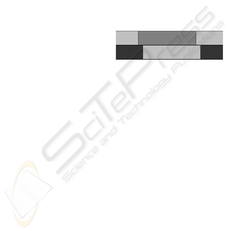
b
d e
Figure 1: A spike is produced when the presynaptic neuron
fires and is sent to a dendrite (a). The dendrite sums up the
weighted spikes (b, equation 1) and calculates its output (c,
equation 2). The postsynaptic neuron sums up the weighted
output of all of its dendrites (d, equation 3) and calculates
its new potential (e, equation 4).
As experience based learning is meant to use past
events to correct and optimise the behaviour, we need
a measurement of error or its equivalent if the former
is not directly available. We have chosen as an al-
ternative to an error value one or more reward values
that can be fed into the control system to represent the
“well-being” of the robot.
These reward values can be modified by positive
“good experience” or negative “bad experience” feed-
back relative to the robot’s performance in the task
that has been assigned. The positive experience is to
be maximised.
In our model we have a single reward value that
represents the general “well-being” of the robot. Its
range is kept from -1, very bad, to 1, very good. The
calculation of the reward can be varied. Usually it
combines current measurements like fast movement,
crashes or the energy level with residual effects of re-
cent ones to avoid too rapid changes. For example,
if the robot crashes into an object, the value for rep-
resenting its “well-being” will be negative for a short
while. A robot that moves away from a obstacle after
crashing into it deserves an increase of the reward.
For the methods that are explained here it is as-
sumed to have a meaningful global reward value Π(t)
at each time step t. This value can be added to a learn-
ing rule as an additional factor. Different authors, all
of them using different neuron functions and learn-
ing functions, have shown that this surprisingly sim-
ple method can successfully be used to implement
reinforcement learning in a neural network (Daucé
and Henry, 2006) (Florian, 2005) (Izhikevich, 2007).
They do not need an external module that evaluates
and changes the connections of the network after each
processing step any more.
ICINCO 2008 - International Conference on Informatics in Control, Automation and Robotics
328
An example for adapting axons and dendrites using
Activation Dependent Plasticity is shown below. Ac-
tivation Dependent Plasticity is based on Hebb’s ideas
of strengthening connections that fire together (Hebb,
1949). As shown by Izhikevich reward can also be in-
tegrated into the more sophisticated Spike Time De-
pendent Plasticity (STDP) learning model (Izhike-
vich, 2007).
Adaptation of an axon weight:
w
a
(t + 1) = w
a
(t) + η
a
· Π(t) · φ
a
· O
d
(5)
where w
a
(t) and w
a
(t + 1) are the axon weights be-
fore and after the adaptation. η
a
is the learning factor
for axons and O
d
is the recent output of the connected
dendrite. φ
a
shows if the axon was active shortly be-
fore the postsynaptic neuron fired. For STDP this
value can be the result of a function that takes into
consideration the time when spikes were transmitted
via the axon. In any case φ
a
is a value from 0 to 1.
Π(t) is the current reward. If it is positive, the
strength of the axon will increase. A negative value
will decrease the strength of the axon.
Adaptation of a dendrite weight:
w
d
(t + 1) = w
d
(t) + η
d
· Π(t) · φ
d
(6)
where w
d
(t) and w
d
(t + 1) are the dendrite weights
before and after the adaptation. η
d
is the learning fac-
tor for dendrites and φ
d
is the activity value of the
dendrite. φ
d
is the equivalent of φ
a
, but φ
d
represents
the activity of the dendrite.
With this function, active excitatory dendrites are
strengthened and active inhibitory dendrites are weak-
ened, if the current reward Π(t) is positive. Otherwise
excitatory dendrites are weakened and inhibitory den-
drites are strengthened.
3.2 Delayed Feedback
In robotics and maybe other real-time control appli-
cations it is very important to consider delayed senso-
rial and perception issues when dealing with feedback
from the environment and ensuing rewards. When
weights are adapted and as discussed later also neu-
rons are created on the controller based on the cur-
rent reward, this may be a problem. Typically, sen-
sor based feedback is received some time after the re-
sponsible action has been decided and executed. De-
pending on the task the robot is performing, the time
differences can vary significantly.
There are two components to consider for tackling
this issue efficiently:
• Feedback is not fed directly into the neural net-
work but just changes the current reward value,
which also contains residual effects of past feed-
back. This avoids fast changes of the reward
value, which would be difficult to assign to a cer-
tain neuron activity pattern.
• In spiking neural networks, there is no single
event that is responsible for an action, but a con-
tinuous flow of spikes. In control terms, this is
equivalent to having the integral element of a PID
scheme; this acts as an embedded filter that makes
that the input pattern, and hence the spiking pat-
tern, does not change rapidly if a certain feedback
is received. Figure 2 shows an example situation
for this issue.
A
B
C
D
E
Action 1
Feedback 3
Action 2
Feedback 2
Action 3
Feedback 1
Figure 2: Section A in the figure illustrates any previous
action of the robot, for example “turning right”. In section
B the robot has started a new action like “moving forward”
but still receives the feedback that should be assigned to the
previous action. Section C shows the time when feedback
is correctly assigned to the current action. In section D the
next action has already started but the feedback is the reac-
tion to action 2. Section E completely belongs to the next
action. Sections B and D, where feedback is not assigned
correctly, are very short compared to the other sections.
In many robotics situations it is still difficult to as-
sign the feedback correctly, for example if there is a
big time difference between action and feedback, or
if there are many concurrent tasks with opposite ac-
tions or feedback values at the same time. However,
even humans do not always arrive at the correct con-
clusions and therefore, although is our aim for robots
to deal with very complex relations, it is not realistic
to expect it to happen with all.
In further work, a method will be introduced that
may enable a robot to deal with delayed feedback in
a better way, or may even be used to predict feed-
back. The method will be refined through further ex-
perimentation and research.
4 NEURAL CONTROLLER
CONSTRUCTION
The neural network to be grown to create a robot con-
trol system initially has no links from the input to the
output. The developer only defines the input neurons
and how they are fed with signals to produce spikes,
the output neurons and how their signals are used, and
SELF CONSTRUCTING NEURAL NETWORK ROBOT CONTROLLER BASED ON ON-LINE TASK
PERFORMANCE FEEDBACK
329

how the global reward is calculated. An example for
how this is done is explained in section 5.
If a non-input neuron has got no predecessors
(neurons, which it gets spikes from), it creates a new
excitatory dendrite and connects it to any neuron. In
the experiments that are discussed later a predecessor
is looked for that is positioned above the postsynaptic
neuron in a layered network structure. Excitatory den-
drites can also look for new presynaptic neurons every
now and then and connect them with weak strength
(low weights). That way a new connection does not
abruptly change an established behaviour.
The method to grow new axons, which are the
connections between presynaptic neurons and den-
drites, can only be used for the action selection task.
To classify different input patterns a method that
creates new neurons is presented. Liu, Buller and
Joachimczak have already shown that correlations be-
tween certain input patterns and a certain reward can
be stored by creating new neurons (Liu and Buller,
2005) (Liu et al., 2006).
In the model proposed here, if the current reward
is positive, a neuron that was active recently should be
active again in similar situations, because, if a certain
action was responsible for positive reward, it may be
successful again. In section 3 delayed feedback was
discussed. To avoid wrong correlations between feed-
back and neuron activity, a neuron will only create a
connection to a new neuron in the following way, if it
was active for some time already:
• All axons with enough influence on a neuron that
was active before receiving positive feedback are
redirected to a new neuron. The influence depends
on the axon weights and the recent activity of the
presynaptic neurons.
• The redirected connections are no longer just ax-
ons to one dendrite but are all connected to their
own dendrite at the new neuron. This stores the
combination of input signals.
• The old axons need not be removed completely,
but most of their strength will be moved to a new
axon that is connected to the new neuron.
• The process, which is illustrated in figure 3, is re-
peated for all dendrites of a neuron.
For a negative reward the process of creating a new
neuron is similar, but the new neuron is not connected
by a new axon but by a new inhibitory dendrite. In
the future a similar input pattern will then inhibit the
neuron that was active before receiving negative feed-
back. Bad actions will be suppressed that way.
Figure 3: The excitatory dendrite a is connected to two neu-
rons of the input layer A via the axons b and c. Both were
active when there was a significant positive reward. A new
neuron was created in the hidden layer B that connects the
same input neurons by two dendrites (d, e) and one axon for
both dendrites (f, g). Then the new neuron was connected
to dendrite a (axon h) of the neuron in the output layer C.
5 EXPERIMENTAL SETUP
Our novel methodology for autonomously construct-
ing a spiking neural network based controller from
a basic initial definition structure was tested with a
simulation of a Pioneer Peoplebot which moves us-
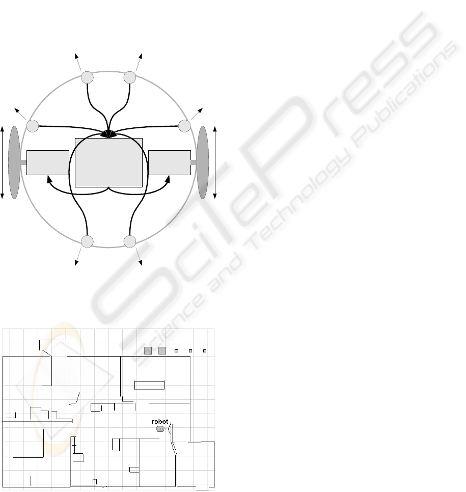
ing differential steering, as depicted in figure 4. The
initial neural structure consists of 12 input neurons (2
for each sensor), 4 output neurons (2 for each motor),
and no connections as indicated by layers A and C in
figure 3.
The input neurons are fed by values from 6 sonar
sensors as shown in figure 4, each sensor feeds the
input of 2 neurons. The sonar sensors are arranged
so that 4 scan the front of the robot and 2 scan the
rear as shown in the figure. The distance value is
processed so that one input neuron fires more fre-
quently as the measured distance increases and the
other neuron connected to the same sensor fires more
frequently as the distance decreases.
For the actuator control, the output connections
are configured so that the more frequently one of
the output neurons connected to each motor fires, the
faster this motor will try to drive forward. The more
frequently the other output neuron connected to the
same motor fires, the faster that motor will try to turn
backward. The final speed that each motor will drive
is calculated by the difference between both neurons.
With the sensor and actuator configuration de-
scribed, the experiment was setup for the robot to
learn to wander around randomly in the simulated of-
fice shown in figure 5 while avoiding obstacles.
In each control cycle the global reward value is
updated along with the processing of the whole sim-
ulated system and movement of the robot. The orig-
ICINCO 2008 - International Conference on Informatics in Control, Automation and Robotics
330
inal Peoplebot’s bumpers are included in the simula-
tion and are used to detect collisions with obstacles,
and are used to penalise significantly the reward val-
ues when such a collision occurs. The reward is in-
creased continuously as the robot travels farther dur-
ing its wandering behaviour. Backward movement
should only be acceptable when recovering from a
collision, therefore it will only be used to increase the
robot’s reward value in that case, while it is used to
decrease this value for all other cases. The straighter
the robot goes the more positive reward it will receive.
So in the long run straight movement will be prefered
compared to moving in circles.
A B
C D
E F
G H
Input neurons
Neural network
Output neurons
Figure 4: The robot interface includes sonar sensors A to F
and motors G and H.
Figure 5: A simulated Peoplebot is situated in this simulated
office provided by MobileRobots/ActivMedia.
Once the controller starts to create connections
and new neurons, they are organised in layers as in-
dicated in figure 3. One layer contains the input neu-
rons and output neurons are located at the layer in the
opposite end. New layers can be created in-between
these two to accommodate new neurons. For these
experiments the network is evaluated as a strict feed
forward network, which means that there are no con-
nections to neurons from the same layer (i.e. no local
inhibition) or to neurons from a previous layer (i.e. no
recurrent connections).
For all experiments Activation Dependent Plas-
ticity was used. That means actions are selected
based on co-activation of certain neurons without con-
sidering the exact spike times. This is suitable for
these experiments where the robot needs to exhibit
a purely reactive behaviour; therefore constraints are
accepted in terms of having no competing actions
that need executing in parallel and without planning
tasks where a sequence or time synchronous actions
need to be executed. Similarly, although advantages
of spike time dependent processes have for example
been investigated by Izhikevich (Izhikevich, 2006) or
van Leeuwen (van Leeuwen, 2004), the learning and
growing mechanisms are not based on such times to
make evaluation easier.
From the explanation of the process to create new
neurons presented in section 4, an additional issue
had to be considered to avoid the creation of large
sequences of neurons when a particular high reward
value is received from the feedback system. When a
new neuron that stores an input pattern that seems to
be responsible for a certain reward value is created,
itself will again generate a reason to produce another
neuron because its output can also be assigned to a
certain reward. To avoid this, the age of the connec-
tions is considered so that young axons, even if they
seem to be responsible for a lot of reward, will not
lead to a new neuron. The effect of this can be ob-
served in Figure 6 where a growing process with and
without this consideration is shown. Without consid-
ering the age of the connections the neural network is
growing so fast that the time needed for all calcula-
tions of one time step increases enormously. Ignoring
young connections saves an extreme amount of new
neurons and also connections.
6 ANALYSIS OF RESULTS
Various experiments were run and consistent results
were obtained where the robot was able to learn au-
tonomously to wander around while turning away
from obstacles. Figure 7 shows an example run in
SELF CONSTRUCTING NEURAL NETWORK ROBOT CONTROLLER BASED ON ON-LINE TASK
PERFORMANCE FEEDBACK
331
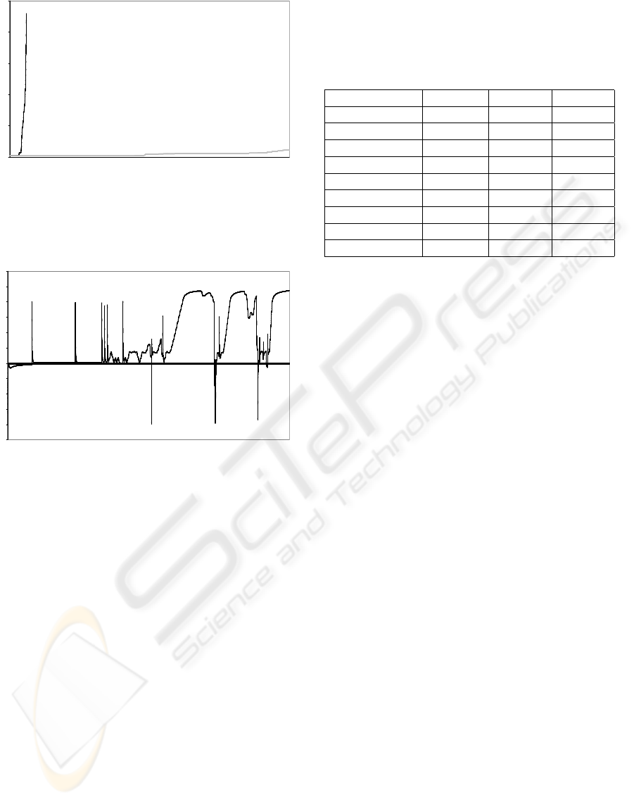
0
500
1000
1500
2000
2500
1
387
773
1159
1545
1931
2317
2703
3089
3475
3861
4247
4633
5019
5405
5791
6177
6563
6949
7335
7721
8107
8493
8879
9265
9651
10037
10423
10809
11195
11581
11967
12353
12739
13125
13511
13897
14283
14669
Time steps
Neurons
Figure 6: The black line shows the number of neurons with-
out considering the age of the connections for creating new
neurons. For the grey line connections younger than 6000
time steps were ignored at the growing process.
-1
-0,8
-0,6
-0,4
-0,2
0
0,2
0,4
0,6
0,8
1
1,2
1
509
1017
1525
2033
2541
3049
3557
4065
4573
5081
5589
6097
6605
7113
7621
8129
8637
9145
9653
10161
10669
11177
11685
12193
12701
13209
13717
14225
14733
15241
15749
16257
16765
17273
17781
18289
18797
19305
19813
Time steps
Reward
Figure 7: At the beginning the robot did not perceive very
much reward. After some random movements the robot
learned how to increase positive reward. Smaller reward
at later stages shows that the robot slowed down near ob-
stacles. The negative amplitudes show that not all obstacles
could be avoided.
which the robot perceived more reward when its ex-
perience increased.
The trend of reward seen in figure 7, where the
feedback varies significantly from high to negative
might look obvious, but it is critical for the robot to
be capable of continuous adaptation. A monotonic in-
crease in the suitability of the system, as is achieved
with other machine learning approaches, would mean
that once the controller learns to perform a task, it
cannot re-adapt to any alteration. This supports fur-
ther the suitability and potential of our novel feedback
guided methodology for autonomously creating robot
controllers.
Table 1 shows some results of a test sample of
50 simulation runs, each run starting with the initial
network definition and without connections, the sys-
tem executed 20000 time steps, where one time step
is over when all neurons have been updated once.
The speed values are measured in internal simulation
units. In all cases, the same number of inhibitory ax-
ons as inhibitory dendrites were created, because as
explained in section 4 a new inhibitory axon is always
created with a new dendrite.
Table 1: The table shows results of 50 simulation runs.
Min. Max. Avg.
Total reward −164.96 7412.83 3160.72
Avg. reward −0.01 0.37 0.16
Max. speed 395.00 1303.00 970.38
Avg. speed 4.09 388.24 190.48
Crashes 0.00 16.00 3.36
Neurons 16.00 32.00 20.62
Exc. axons 14.00 126.00 34.46
Exc. dendrites 4.00 96.00 18.98
Inh. axons 4.00 6.00 4.12
As the system responds autonomously to the feedback
received in the form of reward, it is possible to add or
remove neurons to the input or output layers at any
time, associated either to existing or new sensors and
actuators. The controller will continue to receive the
feedback and continue to adapt autonomously. This
provides a very powerful potential for online adapta-
tion to both new situations and new configurations of
the robot’s hardware. Even in non-explicit situations,
such as standard wear and tear of the system or degra-
dation and failure of a particular component (sensor
or actuator), as long as the task is still possible to be
achieved, the controller will adapt to it.
There is some potential for improving the methods
for the robot to learn to recover if it crashes into an
object. The different parameters of the neural network
have to be adjusted and tested to render the strengths
and weaknesses of the proposed robot control system
more precisely.
7 CONCLUSIONS
We have shown that a robot controller can be created
autonomously using our novel methodology. A neural
network can be grown based on the reward measured
by a feedback function which analyses in real time the
performance of a task.
We have defined a novel methodology where the
design of a robot controller is defined in a completely
new way: as an intuitive process where all that is
required is to identify the inputs, the outputs and
the mechanism to quantify a reward perception from
feedback that depends on the performance of the sys-
tem carrying out a task.
In addition, since the complete process is inte-
grated in a single and robust stage capable of learning
ICINCO 2008 - International Conference on Informatics in Control, Automation and Robotics
332

from experience in a continuous way when running,
this methodology has the potential to be an adaptable
system where we can add or remove any sensors or
actuators, and the controller can adapt autonomously
and online to the new situation.
8 FURTHER WORK
The different parameters that define the speed of
adapting connection weights and the way of creating
new neurons and connections have to be investigated
further to evaluate our novel methodology for creat-
ing controllers for concurrent tasks. These investiga-
tions will lead us to find an elaborate but still very
basic “artificial brain” model that enables a system to
achieve a sophisticated level compared to other artifi-
cial intelligence models by learning from experience
efficiently.
When the basic methods are investigated in detail,
some extensions can be added like Spike Time Depen-
dent Plasticity or a feedback prediction mechanism.
Initial ideas for both enhancements were discussed in
this paper. Those improvements would help the con-
trolled systems to deal with more complex situations,
especially when timing considerations are important.
As mentioned in section 3 assigning delayed feed-
back more efficiently or even predicting feedback will
be an interesting research issue for future work. The
idea is that a neuron that receives positive or nega-
tive reward very often when it is active will probably
receive the same reward also in the future. Predict-
ing reward could actually be one reason for producing
reward. This earlier reward may now be correlated
to the activity of another neuron. That neuron could
again produce reward when predicting it. By the re-
cursive process reward could potentially be predicted
progressively earlier.
REFERENCES
Daucé, E. and Henry, F. (2006). Hebbian learning in large
recurrent neural networks. Technical report, Move-
ment and Perception Lab, Marseille.
Elizondo, D., Fiesler, E., and Korczak, J. (1995). Non-
ontogenetic sparse neural networks. In International
Conference on Neural Networks 1995, IEEE, vol-
ume 26, pages 290–295.
Florian, R. V. (2005). A reinforcement learning algorithm
for spiking neural networks. In Proceedings of the
Seventh International Symposium on Symbolic and
Numeric Algorithms for Scientific Computing, pages
299–306.
Gers, F. A., Schraudolph, N. N., and Schmidhuber, J.
(2002). Learning precise timing with LSTM recurrent
networks. Journal of Machine Learning Research,
3:115–143.
Gómez, G., Lungarella, M., Hotz, P. E., Matsushita, K.,
and Pfeifer, R. (2004). Simulating development in
a real robot: On the concurrent increase of sen-
sory, motor, and neural complexity. In Proceedings
of the Fourth International Workshop on Epigenetic
Robotics, pages 119–122.
Hebb, D. O. (1949). The Organization of Behaviour: A
Neuropsychological Approach. John Wiley & Sons,
New York.
Izhikevich, E. M. (2006). Polychronization: Computation
with spikes. Neural Computation, 18:245–282.
Izhikevich, E. M. (2007). Solving the distal reward prob-
lem through linkage of STDP and dopamine signaling.
Cerebral Cortex, 10:1093–1102.
Katic, D. (2006). Leaky-Integrate-and-Fire und Spike Re-
sponse Modell. Technical report, Institut fï¿
1
2
r Tech-
nische Informatik, Universitï¿
1
2
t Karlsruhe.
Liu, J. and Buller, A. (2005). Self-development of motor
abilities resulting from the growth of a neural network
reinforced by pleasure and tension. In Proceedings of
the 4th International Conference on Development and
Learning 2005, pages 121–125.
Liu, J., Buller, A., and Joachimczak, M. (2006). Self-
motivated learning agent: Skill-development in a
growing network mediated by pleasure and tensions.
Transactions of the Institute of Systems, Control and
Information Engineers, 19(5):169–176.
van Leeuwen, M. (2004). Spike timing dependent structural
plasticity in a single model neuron. Master’s thesis,
Intelligent Systems Group, Institute for Information
and Computing Sciences, Utrecht University.
Vreeken, J. (2003). Spiking neural networks, an introduc-
tion. Technical report, Intelligent Systems Group,
Institute for Information and Computing Sciences,
Utrecht University.
SELF CONSTRUCTING NEURAL NETWORK ROBOT CONTROLLER BASED ON ON-LINE TASK
PERFORMANCE FEEDBACK
333
