RECURSIVE BIAS-COMPENSATING ALGORITHM FOR THE

IDENTIFICATION OF DYNAMICAL BILINEAR SYSTEMS IN THE

ERRORS-IN-VARIABLES FRAMEWORK

T. Larkowski, J. G. Linden, B. Vinsonneau and K. J. Burnham

Control Theory and Applications Centre, Coventry University, Prior Street, Coventry, U.K.

Keywords:

Bias compensation, Bilinear systems, Errors-in-variables, Recursive estimation, Regularization, System iden-

tiﬁcation.

Abstract:

The paper investigates a recursive approach for the bias compensating least squares (BCLS) technique. The

method presented is applied to the problem of on-line identiﬁcation of single-input single-output bilinear

models in the errors-in-variables framework. Within this framework the recursive bilinear BCLS algorithm is

realized when a bilinear Frisch scheme (BFS) is iteratively applied for the estimation of the parameters of an

exemplary bilinear system, giving rise to the exact recursive BFS (ERBFS) method. Moreover, a further exten-

sion of the ERBFS incorporating Tikhonov regularization with variable exponential weighting is considered

and this is shown to be beneﬁcial in the initial period of the identiﬁcation procedure.

1 INTRODUCTION

The errors-in-variables (EIV) framework addresses

the identiﬁcation of dynamical systems where both

the input and the output signals are corrupted by the

measurement noise (S¨oderstr¨om, 2007). The EIV ap-

proaches are found to be of considerable beneﬁt when

the underlying physical laws characterizing the sys-

tem are of a prime interest, as opposed to the predic-

tion of the external signals (S¨oderstr¨om et al., 2002).

In this case, the classical methods based on the least

squares (LS) principle such as recursive LS (RLS)

or the Kalman ﬁlter (Ikonen and Najim, 2002) are

shown to yield estimates of the system parameters that

are asymptotically biased and, therefore, inconsistent

(Zheng, 1998; S¨oderstr¨om, 2007).

In the ﬁeld of modelling for nonlinear systems, the

bilinear system (BS) models have been used to ad-

vantage in various practical applications, e.g. control

plants, biological and chemical phenomena, earth and

sun science, nuclear ﬁssion, fault diagnosis and su-

pervision, see (Mohler, 1991; Mohler and Khapalov,

2000) or (Ekman, 2005). Due mainly to the fact that

BS models are so widely applicable has prompted the

need to extend the EIV approaches developed for lin-

ear systems to encompass the BS case.

Recently, a technique for off-line compensation

of the bias in the case of dynamical BS, i.e. the bi-

linear bias compensating LS (BBCLS) scheme has

been proposed (Larkowski et al., 2007), upon which

a bilinear Frisch scheme (BFS) has been constructed

(Larkowski et al., 2008). The focus of this paper is

the extension of the BBCLS along with the BFS for

the purpose of on-line system identiﬁcation. The pro-

posed approach consists of a recursively performed

update and bias compensation procedure for the data

covariance matrices, whilst the BFS equations are ap-

plied in an iterative manner at each recursion step.

Moreover, a further extension of the BFS incorporat-

ing the Tikhonov regularization (TR) technique with

a variable exponential weighting is considered. It is

shown via simulation studies that use of TR can be of

considerable beneﬁt in the initial period of the identi-

ﬁcation procedure.

The paper is organized as follows: in the second

section the mathematical representation of the EIV

BS together with the assumptions stated and the no-

tation used are introduced. The third section presents

a brief review of the BBCLS and the BFS techniques.

In section four a recursive implementation of the BB-

CLS method is proposed. Subsequently, within the

BBCLS framework the BFS technique is applied re-

sulting in the exact recursive BFS (ERBFS) algo-

rithm. The section ends with an extension of the

ERBFS that incorporates the TR technique. Section

ﬁve presents the results of a numerical simulation

study involving the proposed algorithms, whilst the

overall conclusions and the further work are summa-

rized in section six.

Larkowski T., G. Linden J., Vinsonneau B. and J. Burnham K. (2008).

RECURSIVE BIAS-COMPENSATING ALGORITHM FOR THE IDENTIFICATION OF DYNAMICAL BILINEAR SYSTEMS IN THE ERRORS-IN-

VARIABLES FRAMEWORK.

In Proceedings of the Fifth International Conference on Informatics in Control, Automation and Robotics - SPSMC, pages 38-45

DOI: 10.5220/0001496000380045

 SciTePress

˜u

˜y

Bilinear

system

Figure 1: The basic setup for the EIV BS.

2 ASSUMPTIONS AND

NOTATION

Consider a discrete time-invariant single-input single-

output (SISO) class of BS that can be represented by

the following input/output difference equation

A(q

−1

=B(q

−1

∑

i=1

∑

j=1

k−i

k− j

(1)

with the polynomials A(q

−1

) and B(q

−1

) given by

A(q

−1

) ,1 + a

−1

+ ... + a

−n

(2a)

B(q

−1

) ,b

−1

+ ... + b

−n

(2b)

where r ≤ n

, p ≤ n

≤ n

, q

−1

is the backward shift

operator, deﬁned by x

−1

, x

k−1

and u

, y

are the

noise-free input and output sequences, respectively. A

diagrammatic illustration of the typical EIV setup for

a SISO BS is depicted in Figure 1.

The BS can be classiﬁed into three main cate-

gories, see (Pearson, 1999) for more details, namely:

a) subdiagonal η

= 0 ∀ j > i; b) diagonal η

0 ∀ j 6= i; and c) superdiagonal η

= 0 ∀ j < i. Noting

that both the subdiagonal and superdiagonal cases in-

clude the diagonal case, reference will be solely made

here to the diagonal BS (DBS) case for the remainder

of the paper. This is due to the fact that DBS exhibit

some crucial properties of interest, see (Rao and Gabr,

1984; Liu, 1992) or (Kotta and Nomm, 2003) for a de-

tailed discussion. At the same time DBS are possibly

the most commonly utilized class of BS for the pur-

pose of industrial applications, see (Burnham, 1991;

Yu, 1996; Martineau et al., 2004).

Without loss of generality, the case when all the

diagonal terms in the system (1) are present is consid-

ered here with their number given as n

= p

where

r = p. The following assumptions are introduced:

A1. The DBS is time-invariant, asymptotically stable,

strictly stationary, observable and controllable.

A2. The system structure, i.e. n

, n

, p, is known a

priori.

A3. The true input u

∼ N (0, σ

) is white, persis-

tently exciting and of sufﬁciently high order.

A4. Corrupting input/output noises ˜u

∼N (0,σ

˜u

) and

˜y

∼ N (0,σ

˜y

) of unknown variances are addi-

tive, white, mutually uncorrelated and uncorre-

lated with the noise free signals u

and y

, re-

spectively.

Acknowledging A4, it is implied that the measured

input and output can be decomposed into their noise

free and noise contributions, i.e.

+ ˜u

(3a)

+ ˜y

(3b)

where k denotes the discrete time index. The identiﬁ-

cation problem consists of determining the vector



˜u

˜y



∈ R

(4)

where θ ∈ R

is the parameter vector with n

+ n

and σ

˜u

, σ

˜y

are the input and output noise

variances, respectively. The parameter vector is de-

ﬁned as:

θ ,









a ,













b ,













η ,













(5)

with a ∈ R

, b ∈ R

, η ∈ R

where the extended

parameter vector

θ is given by

θ ,





¯a





∈ R

¯a ,





∈ R

(6)

The regressor vectors for the measured data, noise-

free data and noise are deﬁned, respectively, as:













0,k













(7)

where







−y

k−1

−y

k−n













k−1

k−n













k−1

k−p







RECURSIVE BIAS-COMPENSATING ALGORITHM FOR THE IDENTIFICATION OF DYNAMICAL BILINEAR

SYSTEMS IN THE ERRORS-IN-VARIABLES FRAMEWORK

0,k







−y

k−1

−y

k−n







0,k







k−1

k−n







0,k







k−1

k−p













− ˜y

k−1

˜y

k−n













˜u

k−1

˜u

k−n













k−1,k−1

k−p,k−p







with ϕ

, ϕ

∈ R

, ϕ

0,k

∈ R

, ϕ

0,k

∈ R

, ϕ

0,k

∈ R

and

k−i,k− j

denoting the noise contribution corresponding to the

bilinear product terms of the regressor vector ϕ

. In

agreement with (7), the extended regressor vectors are

given by



−y





−y





− ˜y



(8)

where

∈ R

3 A BRIEF REVIEW OF BBCLS

AND BFS

3.1 BBCLS

The BBCLS algorithm for the class of DBS comprises

of equations (9), (10) and (11), see (Larkowski et al.,

2007). These correspond to the bilinear bias compen-

sation rule, the noise covariance matrix and the noise

‘variance’ of the bilinear terms, respectively, i.e.

BBCLS



ϕϕ

− Σ



−1

ϕy

(9)





˜y

0 0

0 σ

˜u

0 0 σ





(10)

, σ

˜y

+ σ

˜u

− σ

˜u

˜y

(11)

where σ

, E[u

] and σ

, E[y

] are the expected val-

ues of the measured system input and output signals

and (ˆ·) denotes an estimate. It is noted, that in the re-

mainder of the paper, the expression Σ

will be used

as general notation for the correlation matrix of vec-

tors a

and b

, i.e. Σ

= E[a

]. Equation (9) can

be alternatively restated as

BBCLS

+ Σ

−1

ϕϕ

BBCLS

(12)

where

denotes the LS estimate. It is implied from

the BBCLS algorithm that the knowledge regarding

noise variances corrupting input/output of a system

together with variances of measured input/output sig-

nals is sufﬁcient to obtain unbiased estimates of the

true system parameters.

3.2 BFS

The Frisch scheme is a technique that allows the di-

rect estimation of the input/output noise variances to-

gether with the parameters of a system (Beghelli et al.,

1990; S¨oderstr¨om, 2006). As consequence, the a pri-

ori knowledge regarding the values of σ

˜u

and σ

˜y

not required leading to a wider practical applicabil-

ity. The extension of the FS, in the framework of the

BBCLS technique, for the class of DBS has been pro-

posed in (Larkowski et al., 2008). Deﬁne the parti-

tioned extended data covariance matrix









(13)

where Σ

∈ R

+1)×(n

+1)

, Σ

∈ R

×(n

+1)

∈ R

×n

, Σ

∈ R

×(n

+1)

, Σ

∈ R

×n

and Σ

∈ R

×n

. The BFS consists of three main

phases, i.e. calculation of the maximal admissible

value for σ

˜u

, denoted σ

max

˜u

(14), determination of a

functional relationship between σ

˜y

and σ

˜u

(16a) and

the speciﬁcation of a cost function to ﬁnd a unique

value of σ

˜u

(18a). The quantity σ

max

˜u

is given by:

max

˜u

, λ

min

∗

) (14)

where λ

min

∗

) denotes the least eigenvalue of the

matrix A

∗

, and max(·) is the maximum operator. The

matrix A

∗

is deﬁned as:

∗

, A

− B

−1

(15a)

with









(15b)

The functional relationship between σ

˜y

and σ

˜u

described by

˜y

, λ

min

∗

) (16a)

where

∗

, A

−B

(Σ

−σ

˜u

)

−1

(16b)

with



−σ

˜u







(16c)

The cost function utilized is based on the Yule-

Walker equations, see (Diversi et al., 2006) for de-

tails. The instrumental vector (S¨oderstr¨om and Sto-

ica, 1994) for the measured data is deﬁned as:

k−n

−1

∈ R

θ+1

×1

(17)

Using (17) the corresponding cost function is formu-

lated as:

θ) , kΣ

θk

(18a)

such that

θ) = 0 ⇔

θ =

θ (18b)

ICINCO 2008 - International Conference on Informatics in Control, Automation and Robotics

Table 1: Summary of the ERBFS algorithm.

Step Description Procedure

1 Choose λ

and j 0 < λ

< 1, j = 2n

+ 1

2 RLS initialization:

= 0, P

= 10

= 0,

= 0

2.1 RLS loop start for k = n

+ 1... j

2.2 Data weighting γ

= 1/k

Computation of:

2.3 L

, P

k−1

1−γ

k−1

+ L



− ϕ

k−1



1−γ



k−1

− L

k−1



2.4

k−1

2.5 Σ

= Σ

k−1

+ γ



− Σ

k−1



2.6 RLS loop end end

3 BBCLS and BFS initialization Σ

= 0,

max

˜u

= λ

min

∗

1, j

)

3.1 Recursive BBCLS start for k = j+ 1... N

3.2 Data weighting γ

= 1/k

3.3 Iterative BFS start

Computation of:

3.3.1 Σ

= Σ

k−1

+ γ



− Σ

k−1



3.3.2

˜u

= arg min

˜u

)

3.3.3

k−1

3.3.4 Σ

= Σ

k−1

+ γ



− Σ

k−1



3.3.5 A

, B

(Σ

)

−

˜u

, B

(Σ

)

3.3.6 A

∗

2,k

∗

2,k

= A

−B

(Σ

−

˜u

)

−1

)

3.3.7

˜y

= λ

min

∗

2,k

)

3.4 Iterative BFS end

3.5 L

, P

k−1

1−γ

k−1

+ L



− ϕ

k−1



1−γ



k−1

− L

k−1



3.6

˜y

˜u

−

˜u

˜y

3.7 Σ





˜y

0 0

˜u

0 0





3.8 Bias compensation

BBCLS

+ P

BBCLS

k−1

3.9 Recursive BBCLS end end

4 RECURSIVE BBCLS WITH

ITERATIVE BFS

In this section a recursive BBCLS (RBBCLS) algo-

rithm is developed, which comprises the recursive

update of the data and instrumental covariance ma-

trices, whilst the bias compensation procedure is re-

cursively applied to the data covariance matrix only.

Furthermore, an application of the BFS at each iter-

ation step is described with an additional extension

incorporating the TR technique. It is to be noted that

the RBBCLS method can be interpreted in the frame-

work of the iterative bias compensating LS (BCLS)

approaches, see e.g. (Zheng, 1998) and (Zheng, 2000)

for more details.

RECURSIVE BIAS-COMPENSATING ALGORITHM FOR THE IDENTIFICATION OF DYNAMICAL BILINEAR

SYSTEMS IN THE ERRORS-IN-VARIABLES FRAMEWORK

4.1 Recursive BBCLS

The normalized recursive updates of the instrumental

and data covariance matrices are given by the follow-

ing equations, see (Ljung, 1999)

= Σ

k−1

+ γ



− Σ

k−1



(19a)

= Σ

k−1

+ γ



− Σ

k−1



(19b)

with



i=1

k,i



−1

k−1

+ γ

k−1

(20)

where the i-th data is weighted at the discrete time k

according to the following rule

k,i

= λ

k−1,i

for 0 ≤ i ≤ k − 1 (21)

and β

k,k

= 1. It is to be noted that (20) simpliﬁes

either to 1/k in the case of no adaptivity, i.e. when

= 1 or to 1− λ when the exponential forgetting is

used, i.e. λ

= λ with 0 < λ < 1.

Assuming that the input/output noise variances,

i.e. σ

˜u

and σ

˜y

are known a priori or can be estimated,

allows application of the BBCLS algorithm to the re-

cursively computed estimate of the parameter vector,

i.e.

BBCLS

+ P

BBCLS

k−1

(22a)





˜y

0 0

0 σ

˜u

0 0





(22b)

˜y

˜u

− σ

˜u

˜y

(22c)

k− 1

k−1

k− 1

(22d)

k− 1

k−1

k− 1

(22e)

k−1

1−γ

(22f)

k−1

+ L



− ϕ

k−1



(22g)

1− γ



k−1

− L

k−1



(22h)

It is remarked that whilst the input/output noise vari-

ances are postulated to be known, the noise ‘variance’

corresponding to the bilinear terms (22c) is required

to be recursivelyapproximated at each time step. This

involves the recursive estimation of the variances of

the input/output signals, i.e. (22d) and (22e) (Young,

1984). Note that due to assumptions A1 and A3, see

(Pearson, 1999) for more details, the mean values of

the input/output signals do not explicitly appear in ex-

pressions (22d) and (22e) since they are both null.

4.2 Iterative BFS

Utilization of the recursively evaluated data and in-

strumental covariance matrices from the RBBCLS al-

gorithm allows the application of the BFS at each

recursion. Thus it is possible not only to estimate

the input/output noise variances but also to conduct

the noise compensation procedure given by (22a), see

(Linden et al., 2007) for more details regarding the

linear case. This results in the ERBFS algorithm

which is summarized in Table 1. It is to be noted that

ERBFS is rather expensive from the computational

point of view. However, with reference to Table 1, if

the time allowed for the calculation of

˜u

at step 3.3.2

is bounded, the algorithm at least satisﬁes the prin-

ciples of a recursive estimation scheme (Ljung and

S¨oderstr¨om, 1987; Ljung, 1999).

4.3 Regularized BFS

In the case when a priori knowledge regarding the

value of the input noise variance is available,or can be

approximately anticipated, a regularization technique

may be utilized. The regularization method consid-

ered here is that of TR which forces the estimate to-

wards a pre-speciﬁed value

∗

˜u

controlled by the pa-

rameter ω (Hansen, 2001). The incorporation of TR

into the cost function given by (18a) results in the fol-

lowing regularized cost function

θ,ω,

∗

˜u

), ωkΣ

θk

+ (1−ω)k

∗

˜u

−

˜u

(23)

Note that (23) reduces to (18a) for ω = 1. Further-

more, it may be beneﬁcial to consider a variable con-

trolling parameter, i.e. ω

, such that the impact of

the regularization is signiﬁcant at the beginning of the

identiﬁcation procedure but gradually diminishes as a

function of the incoming data stream. It is proposed

to realize the concept as follows

= e

−

(24)

where ς is a user deﬁned parameter describing the rate

at which the impact of the regularization diminishes.

This choice allows the potential bias introduced by

regularization (Hansen, 2001) to be alleviated as time

progresses. With reference to Table 1, the introduc-

tion of regularization requires the additional setting of

the parameter ς at step 3, the subsequent implemen-

tation of equation (24) between steps 3.3.1 and 3.3.2

and replacement of the cost function J

(

) from 3.3.2

by J(

,ω

∗

˜u

ICINCO 2008 - International Conference on Informatics in Control, Automation and Robotics

5 SIMULATION STUDIES

This section provides a numerical evaluation and

comparison of the proposed ERBFS algorithm with

the RLS and the off-line BFS. The SISO DBS system

used in the simulations with n

= 2, n

= n

= 1 is

simulated for N = 5000. It is described by the follow-

ing difference equation

= 1.2y

k−2

− 0.9y

k−1

+ 0.6u

k−1

0.1y

k−1

(25)

The input is generated by

∼ N (0,0.5) (26)

The variances of the input and output noises are

selected as σ

˜u

= 0.05 and σ

˜y

= 0.16, respectively,

in order to yield an approximately equal signal-to-

noise ratio (SNR) on both input and output, i.e.

SNR

≈ SNR

≈ 10[dB]. In the case of the ERBFS

and the regularized ERBFS (RERBFS) the minimiza-

tion procedure from step 3.3.2 (see Table 1) is re-

stricted to a maximum of 10 iterations. The parameter

is set to unity, i.e. no adaptivity, for all evaluated

algorithms.

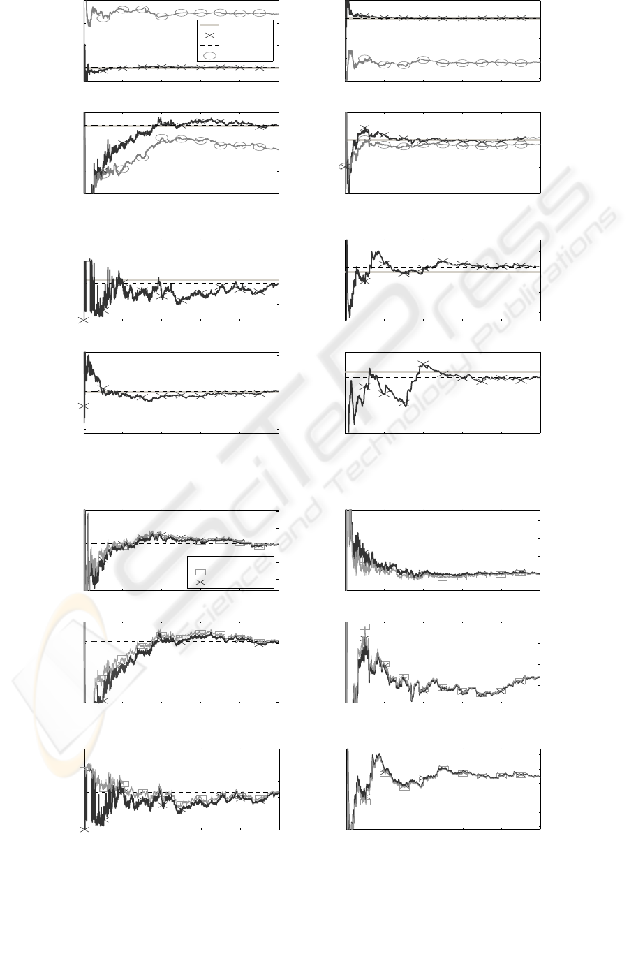
Considering the results presented in Figure 2,

where the ERBFS is compared with its off-line coun-

terpart and the RLS, the following observations are

made:

a) RLS yields estimates that are asymptotically bi-

ased for the case of all system parameters.

b) The estimate of the vector ϑ obtained via the off-

line BFS is quite close to its true value.

c) The EBFS achieved virtually identical estimates

as the off-line BFS at the last recursion step, i.e.

k = N.

d) Estimates given by EBFS converge to their off-

line counterparts obtained by the BFS algorithm

over the succesive recursions.

e) There is a clear correlation between the quality of

the estimated variances of the input/output signals

and the quality of the estimated input/output noise

variances which, subsequently, has an impact on

the estimates of the system parameters.

f) The ERBFS encountered some difﬁculties in the

estimation of the input noise variance in the ini-

tial part of the identiﬁcation procedure, i.e. up to

about ﬁrst 1000 samples which is indicated by the

relatively highly scattered values of

˜u

In fact observation(f) can be regarded as a premise for

considering regularization of the input noise variance

such that the uncertainty in the initial part of the iden-

tiﬁcation is alleviated, leading to improved accuracy

of the estimates. In the second experiment the ERBFS

is compared with the RERBFS, where the parameters

are set as follows: ς = N/ω

where ω

= 100 and

∗

˜u

= 1.5σ

˜u

. For completeness, the results obtained

by the BFS are also included. Consideration of the

results in Figure 3 leads to the following observations:

g) Although the guess of the regularization parame-

ter σ

∗

˜u

was rather ‘rough’, a substantial improve-

ment w.r.t. the input noise variance is observed in

the initial period of the recursion.

h) The impact of applying TR is also evident in the

case of the estimated output noise variance and

the system parameters leading to the faster con-

vergence.

i) Due to the utilization of the exponential control-

ling variable weighting ω

the results obtained by

the RERBFS and ERBFS at k = N are practically

indistinguishable. As a consequence, any poten-

tial induced bias due to the use of regularization

is kept to a minimum, for the case considered.

6 CONCLUSIONS

A new recursive technique, i.e. the RBBCLS method,

for identiﬁcation of the class of SISO DBS has been

developedand evaluated. Within the RBBCLS frame-

work the ERBFS algorithm has been formulated in

which the Frisch equations are evaluated at each re-

cursion. The further extension incorporating the vari-

able regularization via the TR method, giving rise to

the RERBFS, was considered and shown to be bene-

ﬁcial in the initial period of the identiﬁcation proce-

dure. The methods proposed have been demonstrated

when applied to a SISO DBS EIV identiﬁcation prob-

lem. Comparisons made with the standard RLS tech-

nique illustrates the superiority and relatively high

noise robustness of the proposed algorithms.

The further work will address two outstanding is-

sues. Firstly, the extension and subsequent recursive

implementation of the BCLS method to a wider class

of the polynomial nonlinear EIV systems. Secondly,

the alleviation of the computationalburden via the ap-

plication of a fully recursive BFS based on gradient

approaches and/or on other fast methods via lineariza-

tion of the Frisch equations.

REFERENCES

Beghelli, S., Guidorzi, R. P., and Soverini, U. (1990). The

Frisch scheme in dynamic system identiﬁcation. Au-

tomatica, 26(1):171–176.

RECURSIVE BIAS-COMPENSATING ALGORITHM FOR THE IDENTIFICATION OF DYNAMICAL BILINEAR

SYSTEMS IN THE ERRORS-IN-VARIABLES FRAMEWORK

Burnham, K. J. (1991). Self-tuning Control for Bilinear Sys-

tems. PhD thesis, Coventry Polytechnic.

Diversi, R., Guidorzi, R., and Soverini, U. (2006). Yule-

Walker equations in the Frisch scheme solution of

errors-in-variables identiﬁcation problems. In Proc.

of the 17th Int. Symposium on Mathematical Theory

of Networks and Systems, Kyoto, Japan.

Ekman, M. (2005). Modeling and Control of Bilinear Sys-

tems: Applications to the Activated Sludge Process.

PhD thesis, Uppsala University.

Hansen, P. C. (2001). Regularization tools: A matlab

package for analysis and solution of discrete ill-posed

problems. Technical report, Department of Mathemat-

ical Modelling, Technical University of Denmark.

Ikonen, E. and Najim, K. (2002). Advanced Process Identi-

ﬁcation and Control. Marcel Dekker, Inc., USA.

Kotta, U. and Nomm, S.and Zinober, A. (2003). On state

space realizability of bilinear systems described by

higher order difference equations. In Proc. of 42nd

IEEE Conf. on Decision and Control, volume 6, pages

5685–5690.

Larkowski, T., Linden, J. G., Vinsonneau, B., and Burnham,

K. J. (2008). A novel errors-in-variables approach for

bilinear models: the bilinear Frisch scheme. Internal

report no. CTAC/TL-1/2008, Control Theory and Ap-

plications Centre, Coventry University, Coventry.

Larkowski, T., Vinsonneau, B., and Burnham, K. J. (2007).

Bilinear model identiﬁcation in the errors-in-variables

framework via the bias-compensating least squares. In

IAR and ACD Int. Conf., Grenoble, France.

Linden, G. J., Vinsonneau, B., and Burnham, K. J. (2007).

Fast algorithms for recursive Frisch scheme system

identiﬁcation. In IAR and ACD Int. Conf., Grenoble,

France.

Liu, J. (1992). On stationarity and asymptotic inference of

bilinear time series models. Statistica Sinica, 2:479–

494.

Ljung, L. (1999). System Identiﬁcation - Theory for the

User. Prentice Hall PTR, New Jersey, USA, 2nd edi-

tion edition.

Ljung, L. and S¨oderstr¨om, T. (1987). Theory and practice of

recursive identiﬁcation. MIT Press, Cambridge, UK.

Martineau, S., Burnham, K. J., Haas, O. C. L., Andrews,

G., and Heeley, A. (2004). Four-term bilinear pid con-

troller applied to an industrial furnace. Control Engi-

neering Practice, 12(4):457–464.

Mohler, R. R. (1991). Nonlinear Systems: Applications to

Bilinear Control, volume 2. Prentice Hall, Englewood

Cliffs, NJ.

Mohler, R. R. and Khapalov, A. Y. (2000). Bilinear con-

trol and application to ﬂexible a.c. transmission sys-

tems. Journal of Optimization Theory and Applica-

tions, 105(3):621–637.

Pearson, R. K. (1999). Discrete-Time Dynamic Models. Ox-

ford University Press, New York, USA.

Rao, T. S. and Gabr, M. M. (1984). An Introduction to

Bispectral Analysis and Bilinear Time Series Models.

Springer-Verlag, Berlin, Germany.

S¨oderstr¨om, T. (2006). Statistical analysis of the Frisch

scheme for identifying errors-in-variables systems.

Technical report, Upsala Univercity, Department of

Information Technology, Upsala, Sweden.

S¨oderstr¨om, T. (2007). Errors-in-variables methods in sys-

tem identiﬁcation. In Automatica, volume 43, pages

939–958.

S¨oderstr¨om, T., Soverini, U., and Mahata, K. (2002). Per-

spectives on errors-in-variables estimation for dy-

namic systems. In Signal Processing, volume 82(8),

pages 1139–1154.

S¨oderstr¨om, T. and Stoica, P. (1994). System Identiﬁcation.

Prentice Hall Int., New Jersey, USA.

Young, P. (1984). Recursive Estimation and Time-Series

Analysis. Springer-Verlag, Berlin, Germany.

Yu, D. (1996). Fault diagnosis for industrial systems with

emphasis on bilinear systems. PhD thesis, Coventry

University.

Zheng, W. X. (1998). Transfer function estimation from

noisy input and output data. Int. Journal of Adaptive

Control and Signal Processing, 12:365–380.

Zheng, W. X. (2000). Parametric identiﬁcation of linear

noisy input-output systems. Cybernetics and Systems,

31(7):803–816.

ICINCO 2008 - International Conference on Informatics in Control, Automation and Robotics

1000 2000 3000 4000 5000

−1.2

−1.1

−1

−0.9

1000 2000 3000 4000 5000

0.6

0.7

0.8

0.9

1000 2000 3000 4000 5000

0.45

0.5

0.55

0.6

1000 2000 3000 4000 5000

−0.1

0.1

0.2

BFS

ERBFS

true

RLS

1000 2000 3000 4000 5000

0.02

0.04

0.06

0.08

0.1

1000 2000 3000 4000 5000

0.12

0.14

0.16

0.18

1000 2000 3000 4000 5000

0.45

0.5

0.55

0.6

0.65

1000 2000 3000 4000 5000

1.4

1.6

1.8

˜u

˜y

Figure 2: The results of the identiﬁcation procedure using ERBFS, BFS and RLS algorithms.

1000 2000 3000 4000 5000

−1.22

−1.21

−1.2

−1.19

−1.18

1000 2000 3000 4000 5000

0.9

0.91

0.92

0.93

1000 2000 3000 4000 5000

0.5

0.55

0.6

1000 2000 3000 4000 5000

0.1

0.12

0.14

0.16

RERBFS

BFS

ERBFS

1000 2000 3000 4000 5000

0.02

0.04

0.06

0.08

0.1

1000 2000 3000 4000 5000

0.13

0.14

0.15

0.16

0.17

0.18

˜u

˜y

Figure 3: The results of the identiﬁcation procedure using BFS, RERBFS and ERBFS algorithms.

RECURSIVE BIAS-COMPENSATING ALGORITHM FOR THE IDENTIFICATION OF DYNAMICAL BILINEAR

SYSTEMS IN THE ERRORS-IN-VARIABLES FRAMEWORK