CONTROLLING INVESTMENT PROPORTION IN CYCLIC

CHANGING ENVIRONMENTS

J.-Emeterio Navarro-Barrientos

Department of Computer Science, Humboldt-Universit¨at zu Berlin, Unter den Linden 6 10099, Berlin, Germany

Keywords:

Genetic algorithms, investment strategies, pattern recognition.

Abstract:

In this paper, we present an investment strategy to control investment proportions for environments with cyclic

changing returns on investment. For this, we consider an investment model where the agent decides at every

time step the proportion of wealth to invest in a risky asset, keeping the rest of the budget in a risk-free

asset. Every investment is evaluated in the market modeled by stylized returns on investment (RoI). For

comparison reasons, we present two reference strategies which represent agents with zero-knowledge and

complete-knowledge of the dynamics of the RoI, and we consider an investment strategy based on technical

analysis. To account for the performance of the strategies, we perform some computer experiments to calculate

the average budget that can be obtained over a certain number of time steps. To assure for fair comparisons,

we ﬁrst tune the parameters of each strategy. Afterwards, we compare their performance for RoIs with ﬁxed

periodicity (stationary scenario) and for RoIs with changing periodicities (non-stationary scenario).

1 INTRODUCTION

Finding a proper method to control investment pro-

portion is a problem that has been addressed by many

researchers (Kelly, 1956; Kahneman and Tversky,

1979). Many of the proposed methods are based on

machine learning (ML). For example, in (Magdon-

Ismail et al., 2001) the authors use neural networks

to ﬁnd patterns in ﬁnancial time series and in (Geibel

and Wysotzki, 2005), the authors propose a risk-

sensitive reinforcement learning algorithm to ﬁnd

a policy for controlling under constraints. Other

techniques from ML that are also frequently used

are those based on evolutionary computation, like

genetic programming (GP) and genetic algorithms

(GA). For a general introduction to these techniques

for portfolio management and bankruptcy prediction

see (Dawid, 1999). Some researchers have shown that

investment strategies based on GP techniques may be

proﬁtable; however, they usually ﬁnd strategies which

can’t be easily funded (Schulenburg and Ross, 2001).

Controlling strategies that are based on a standard GA

may be also difﬁcult to explain, however, we believe

that they are easier to understand than those using GP.

Genetic algorithms (GA) are stochastic search al-

gorithms based on evolution that explore progres-

sively from a large number of possible solutions ﬁnd-

ing after some generations the best solution for the

problem. Inspired by natural selection, these powerful

techniques are based on some deﬁned evolution oper-

ators, like selection, crossover and mutation (Holland,

1975). Moreover, some researches have extended

the use of GA for solving stochastic dynamic opti-

mization problems online (Grefenstette, 1992), where

most of the algorithms for changing environments are

tested in problems like the knapsack problem (Yang,

2005). However, to our knowledge, no-one has ap-

plied GAs speciﬁcally to the problem of controlling

the proportion of investment in environments with

cyclic changing returns on investment.

This paper is organized as follows: Sec. 2 de-

scribes the investment model and Sec. 3 presents

a novel approach to control investment proportions

based on a GA for environments with cyclic chang-

ing time series. In Sec. 4 we present the dynamics

for the risky asset and we compare the performance

of the adaptive strategy with other strategies for sta-

tionary and non-stationary environments.

2 INVESTMENT MODEL

We consider an investment model (Navarro and

Schweitzer, 2003) where an agent is characterized by

207

Navarro-Barrientos J. (2008).

CONTROLLING INVESTMENT PROPORTION IN CYCLIC CHANGING ENVIRONMENTS.

In Proceedings of the Fifth Inter national Conference on Informatics in Control, Automation and Robotics - ICSO, pages 207-213

DOI: 10.5220/0001496802070213

 SciTePress

two individual variables: (i) its budget x(t), and (ii) its

investment proportion q(t). The budget, x(t), changes

in the course of time t by means of the following dy-

namic:

x(t + 1) = x(t)

1+ r(t)q(t)

(1)

This means that the agent at time t invests a por-

tion q(t)x(t) of its total budget. And this investment

yields a gain or loss on the market, expressed by r(t),

the return on investment, RoI. Some authors assume

that returns are obtained by means of continuous dou-

ble auction mechanisms (LeBaron, 2001), however,

in this paper we consider that the returns are not be-

ing inﬂuenced by agent’s actions, this approach plays

a role in more physics-inspired investment models,

(Richmond, 2001; Navarro-Barrientos et al., 2008).

Since q(t) always represents a portion of the total bud-

get x(t), and it is bound to q(t) ∈ [0,1]. For complete-

ness, we assume that the minimal and maximal in-

vestment proportions are described by q

min

and q

max

respectively.

Thus, in this paper we present an adaptive strat-

egy to control proportions of investment, expressed

by a method to ﬁnd the most proper q(t). We assume

a simple dynamic for the returns allowing us to focus

in the feedback of these market returns on the invest-

ment strategy (and not on the feedback of the strate-

gies on the market). Moreover, we assume that the

agent invests independently in the market, i.e. there is

no direct interaction with other agents.

3 ADAPTIVE INVESTMENT

STRATEGY

In this section, we present an adaptive investment

strategy based on a GA for controlling proportions

of investment in cyclic changing environments. For

simplicity, we call this strategy Genetic Algorithm for

Changing Environments (GACE), and we show on the

following the speciﬁcations for the GA.

3.1 Encoding Scheme

We consider a population of chromosomes j =

1,...,C, where each chromosome j has an array of

genes, g

, where k = 0,...,G

− 1, and G

is the

length of the chromosome j. The length of a chro-

mosome is assumed to be in the range G

∈ (1, G

max

where G

max

is a parameter that speciﬁes the maximal

allowed number of genes in a chromosome. The val-

ues of the genes could be binary, but for program-

ming reasons we use real values (Michalewic¸z, 1999).

Moreover, each chromosome j represents a set of pos-

sible strategies of an agent, where each g

is an in-

vestment proportion.

3.2 Fitness Evaluation

Each chromosome j is evaluated after a given num-

ber of time steps by a ﬁtness function f

(τ) deﬁned as

follows:

(τ) =

−1

∑

k=0

r(t)g

; k ≡ t mod G

, (2)

where τ is a further time scale in terms of genera-

tions. When a generation is completed, the chromo-

somes’ population is replaced by a new population of

better ﬁtting chromosomes with the same population

size C. Since the ﬁtness of a chromosome tends to be

maximized, negative r(t) should lead to small values

of g

, and positive r(t) should lead to larger values

of g

. Because of this, we consider the product of

r(t)g

as a performance measure, which is in accor-

dance with our investment model, Eq. (1). Notewor-

thy, in this approach the GA tries to ﬁnd the chromo-

somes leading to larger proﬁts. A different approach

would be to implement a GA to ﬁnd the chromosomes

that minimize the loss, in which case, we would have

a different ﬁtness function. Note that we treat directly

returns on investment and not price movements, be-

cause our goal is to evaluate the ﬁtness of the strate-

gies for the RoI and not the accuracy of the prediction

of the next RoI.

3.3 Selection of a New Population

If we assume that chromosomes have ﬁxed length,

= G

max

, then the most proper number of time steps

that have to elapse in order to evaluate all chromo-

somes’ genes is t

eval

= G

max

. However, this previous

assumption corresponds to the ideal case where the

agent knows the periodicity of the returns and sets the

length of all chromosomes to this value. In this paper,

we assume that the agent doesn’t know neither the

periodicity nor the dynamics of the RoI. Thus, we

assume that the chromosomes have different length.

Different approaches may be proposed to know after

how many time steps a new generation of chromo-

somes should be obtained, however, we ﬁnd that the

best approach was to choose the number of time steps

for evaluation accordingly to the length of the best

chromosome in the population.

3.3.1 Elitist and Tournament Selection

After calculating the ﬁtness of each chromosome ac-

cording to Eq. (2), we ﬁrst ﬁnd the best chromosomes

ICINCO 2008 - International Conference on Informatics in Control, Automation and Robotics

208

from the current population by applying elitist selec-

tion, which copies directly the best s percentage to the

new population. Afterwards, a tournament selection

of size two is done by randomly choosing two pairs

of chromosomes from the current population and then

selecting from each pair the one with the higher ﬁt-

ness. These two chromosomes are not simply trans-

ferred to the new population, but undergo a transfor-

mation based on the genetic operators’ crossover and

mutation.

3.3.2 Crossover and Mutation Operators

The limitations of conventional crossover in GA with

variable length has already been addressed by some

authors, where neural networks or hierarchical tree-

structures are used to determine which genes should

be exchanged between the chromosomes (Harvey,

1992). For simplicity, we propose a modiﬁcation

of the standard GA crossover operator that better

suits our demands. Thus, we propose the use of

a crossover operator called Proportional Exchange

Crossover (PEC) operator, which randomly selects

the range of genetic information to be exchanged be-

tween two chromosomes and contracts(extends) the

genetic information from the largest(shortest) to the

shortest(largest) chromosome, respectively. Algo-

rithm 1 shows the PEC algorithm for all pair of

parent-chromosomes being selected via tournament

selection. Note that a chromosome j is saved in an

array with indexes in the range [0,..,G

− 1]. The

shortest and largest parent-chromosomes are denoted

by pa

with size G

and pa

with size G

, resp., and

R ∈ N is the size proportion between these two parent-

chromosomes. The cross-points for the shortest and

largest parent-chromosomes are denoted by cp

∈ N

and cp

∈ N, respectively. The breeding between the

two parent-chromosomes results in a short and a large

children-chromosomes denoted by ch

and ch

, re-

spectively.

Note, that different functions could be consid-

ered for the transformation of the genetic material be-

tween chromosomes with different length. For sim-

plicity, we consider in our implementation of the Al-

gorithm 1 in line 9 the function extend(pa,m,R) =

pa[m], which simple copies the genes from the short

parent-chromosome to the large child-chromosome;

and in line 13 the function contract(pa,m,R) =

1/R

∑

m+R

i=m

pa[i], which performs an average over the

genetic material.

Now, to make sure that a population with chromo-

somes of diverse lengths is present, we introduce a

mutation operator for the length of the chromosome.

For this, with probability p

a new length is drawn

randomly and the genetic information of the chro-

Algorithm 1: Proportional Exchange Crossover

(PEC) operator.

foreach pair of parent-chromosomes do1

create ch

and ch

with sizes G

and G

ﬁnd the cross-points:3

∼ U(0,G

− 1); cp

determine size proportion: R = cp

/cp

with p = 0.5 choose side for crossover5

if crossover on the left side then6

extend genes from pa

to ch

for m = 0 to cp

− 1 do

for n = 0 to R− 1 do8

[m· R+ n] ←9

extend(pa

,m,R)

end10

end11

contract genes from pa

to ch

:12

foreach m = 0 to cp

− 1 do

[m] ← contract(pa

,m,R)13

end14

else15

extend as in 9 but for m = cp

to G

− 116

contract as in 13 but for m = cp

to17

− 1

end18

copy remaining genes in pa

and pa

into19

same positions in ch

and ch

, respectively.

end20

mosome is proportionally scaled to the new length,

leading to a new enlarged or stretched chromosome.

The algorithm used for the mutation of the length of

the chromosome is based on the same principle as

the PEC operator. After the crossover and length-

mutation operators are applied, the typical gene-

mutation operator is applied. This means that with a

given mutation probability p

∈ U(0,1), a gene is to

be mutated by replacing its value by a random number

from a uniform distribution U(q

min

max

3.3.3 Strategy Selection and Initialization

For every new generation, the agent takes the set of

strategies g

from the chromosome j with the largest

ﬁtness in the previous generation.

q(t) = g

with l = arg max

j=1,..,C

; k ≡ t mod G

(3)

For the initialization, each g

is assigned a ran-

dom value drawn from a Uniform distribution: g

∼

U(q

min

max

). And for the length of the chromo-

somes, each G

is initialized randomly from a Uni-

form distribution of integers: G

∼ (1,G

max

), where

max

is the maximal allowed chromosome length.

CONTROLLING INVESTMENT PROPORTION IN CYCLIC CHANGING ENVIRONMENTS

209

4 EXPERIMENTAL RESULTS

In this section, we present the environment for the

agent and we analyze the performance of the adaptive

strategy presented above.

4.1 Artiﬁcial Returns

We consider artiﬁcially generated returns which are

driven by the following dynamics:

r(t) = (1− σ)sin



2π



+ σξ, (4)

where the amplitude of the returns depends on the am-

plitude noise level σ ∈ (0,1), and ξ corresponds to a

random number drawn from a Uniform distribution,

ξ ∈ U(−1,1). The periodicity of the returns is drawn

randomly T ∼ U(1, T

max

) and would be present for

a number of t

′

∼ U(1,t

max

) time steps. Thus, σ ac-

counts for the ﬂuctuations in the market dynamics on

the amplitude of the RoI; T

max

accounts for the largest

possible periodicity and t

max

accounts for the max-

imal number of time steps a periodicity can elapse.

Fig. 1 shows an example of the RoI.

0 200 400 600 800 1000

-1

-0.5

0.5

r(t)

Figure 1: Periodic RoI, r(t), Eq. (4) for noise level σ = 0.1,

max

= 100 and t

max

= 1000.

4.2 Reference Strategies

For comparison purposes, we present in this section

different strategies which are used as a reference to

account for the performance of the adaptive strategy.

Note that we could have considered other type of

strategies which may lead to a more complete study.

However,our main goal is to show the performance of

GACE comparing it against the performance of other

strategies for the same investment scenario.

4.2.1 Strategies with Zero/Complete Knowledge

For comparison reasons, we present in this sec-

tion two strategies representing two simple behav-

iors for an agent: the ﬁrst one, called Constant-

Investment-Proportion(CP), represents the agent with

zero knowledge and zero-intelligence; the second

one, called Square-Wave (SW), represents the agent

with complete knowledge of the environment.

Constant Investment Proportion (CP). The sim-

plest strategy for an agent would be to take a constant

investment proportion for every time step:

q(t) = q

min

= const. (5)

Square Wave Strategy (SW). An agent using this

strategy invests q

max

during the positive cycle of the

periodic return and invests q

min

otherwise:

q(t) =

(

max

t mod T < T/2

min

otherwise.

(6)

Notice that this reference strategy assumes that the

agent knows in advance the periodicity, T, and the

dynamics of the returns.

4.2.2 Strategy based on Technical Analysis

We include in our study a strategy based on techni-

cal analysis methods, which are frequently used by

traders to forecast returns. For simplicity, we chose

the Moving Least Squares (MLS) technique and con-

sidered an agent with a memory size M to store previ-

ous received returns. This strategy ﬁts a linear trend-

line to the previous M returns, to estimate the next re-

turn, ˆr(t). Noteworthy, once the next return has been

estimated, the agent still needs to perform the cor-

responding adjustment of the investment proportion.

For this, we consider that the agent has a risk-neutral

behavior as follows:

q(t) =











min

ˆr(t) ≤ q

min

ˆr(t) q

min

< ˆr(t) < q

max

ˆr(t) ≥ q

max

(7)

4.3 Results for RoI with Fixed

Periodicity

To elucidate the performance of the adaptive strat-

egy proposed in this paper and the reference strategies

previously presented, we start with a simple scenario

where returns have a ﬁxed periodicity.

First, we assume that the parameters of a strat-

egy lead to an optimal performance, if it leads to

the maximum total budget that can be reached with

this strategy during a complete period of the returns.

When evaluating the strategies, we have to consider

that their performance is also inﬂuenced by stochas-

tic effects. In the case of the strategy GACE we also

have to account for the different possible strategies

that may evolve. This means that we have to aver-

age the simulation over a large number of trials, N,

where each trial simulates an agent acting indepen-

dently with the same set of parameter values. For con-

venience, we reinitialize the budget after each cycle of

ICINCO 2008 - International Conference on Informatics in Control, Automation and Robotics

210

the RoI. This is done, because if the strategy performs

well, the budget of the agent may reach very high val-

ues, which would lead to numerical overﬂows.

4.3.1 GACE Parameter Tuning

The conﬁguration of most meta-heuristic algorithms

requires both complex experimental designs and high

computational efforts. Thus, for ﬁnding the best pa-

rameters for the GA, a software called +CARPS (Mul-

tiagent System for Conﬁguring Algorithms in Real

Problem Solving) (Monett, 2004) was used. It con-

sists of autonomous, distributed, cooperative agents

that search for solutions to a conﬁguration problem,

thereby ﬁne-tuning the meta-heuristic’s parameters.

The GA was conﬁgured for periodic returns with

T = 100 and different level of noise: σ = 0.1,

and σ = 0.5. Four GA parameters were optimized:

the population size C, the crossover probability p

the mutation probability p

, and the elitism size

s. Their intervals of deﬁnition were set as follows:

C ∈ {50, 100,200,500, 1000}, p

∈ [0.0, 1.0], p

∈

[0.0,1.0], and s ∈ [0.0,0.5]. We show in Table 1 the

best obtained conﬁguration for the GA in the periodic

returns previously mentioned. For clarity, we con-

sidered in these experiments chromosomes with ﬁxed

length, i.e. G

= T, and no probability of length mu-

tation, i.e p

= 0.

Table 1: GACE’s best pars. for RoI with ﬁxed T.

C p

1000 0.7 0.01 0.3

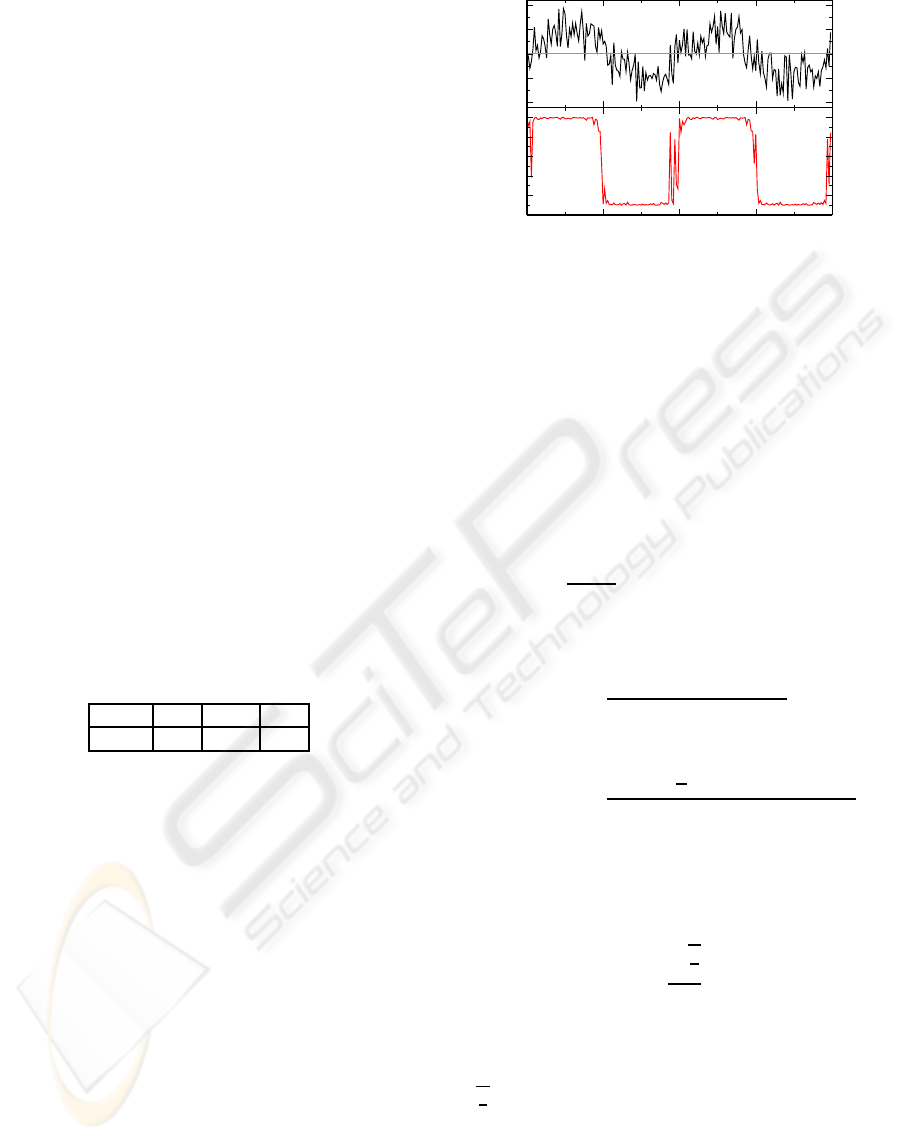
Now, to better illustrate the set of investment

strategies that are being obtained using GACE, we

show in Fig. 2 the RoI and the investment proportions

obtained after a number of time steps. For the reader

with background in signal processing techniques, Fig.

2 may sound familiar as it resembles to those ﬁgures

obtained when using matched ﬁlters for signal recov-

ery (Turing, 1960).

4.3.2 Performance Comparison

In order to assure fair comparison between the strate-

gies, we need to ﬁnd the most proper parameter val-

ues for the strategies. Note that for both strategies CP,

Eq. (5) and SW, Eq. (6), we don’t need to tune any

parameters. However, for the strategy MLS, Eq. (7),

we assume that the agent knows the periodicity T of

the returns. This means that the agent needs to de-

termine the most proper memory size, M, based on

the known periodicity of the returns. For this, we per-

formed some computer experiments using MLS with

-1

-0.5

0.5

r(t)

0.2

0.4

0.6

0.8

q(t)

99800

99850

99900

99950

100000

Figure 2: (Top)Return r(t) and (bottom) investment con-

trol strategy q(t) using GACE after t = 10

time steps, for

returns with T = 100 and σ = 0.5.

different memory sizes for returns with different ﬁxed

periodicities, T, and no noise, ﬁnding that the most

proper memory size, M, and the periodicity, T, are

proportionally related by M/T ≈ 0.37. Now, if we as-

sume returns with no noise, we can ﬁnd analytically

the memory size M

⋆

that maximizes the proﬁts. For

this, it can be shown that for periodic returns as in

Eq. (4) with σ = 0, the strategy MLS, Eq. (7), esti-

mates the next return ˆr(t + 1) as follows:

ˆr(t + 1) =

M + 1

[sin(ωt) − sin(ωt − ωM)], (8)

where ω = 2π/T. Now, by calculating the average

proﬁts hrqi for the positive cycle of the returns:

hrqi =

T (M+ 1− cos(ωM))

. (9)

And obtaining the derivative of hrqi w.r.t M:

∂

hr(t)q(t)i =

−T sin





+ πM sin(ωM)

(10)

It can be shown that by solving ∂

hr(t)q(t)i = 0 and

using Taylor expansion to the sixth order for the sinu-

soidal functions, the memory size M

⋆

that maximizes

the proﬁts corresponds to:

⋆

T. (11)

Consequently, the proportion M/T ≈ 0.37 found

by means of computer simulations approximates

pretty well the proportion found analytically M/T =

/π = 0.389.

Now, we compare the performance of the adap-

tive investment strategy GACE, presented in Sec. 3,

with respect to the reference strategies presented in

Sec. 4.2. For clarity, we assume for the moment that

the strategy GACE uses ﬁxed chromosome length, i.e.

= G

max

. For all strategies we consider q

min

= 0.1

CONTROLLING INVESTMENT PROPORTION IN CYCLIC CHANGING ENVIRONMENTS

211

and q

max

= 1.0 in our experiments. These parame-

ter values describe the behavior of the strategies CP,

Eq. (5), and SW, Eq. (6). For the strategy MLS,

Eq. (7), we use Eq. (11) to determine the optimal

memory size and for the strategy GACE we use the

parameters in Table 1.

In our experiments we assume that the agent in-

vests in returns with periodicity T = 100 for different

noise levels. We consider here that the length of the

chromosomes is ﬁxed to G

= 100 and a new genera-

tion of chromosomes is being obtained after a number

of time steps t

eval

= 100. For the computer experi-

ments, we let the agent to use one of the strategies

to invest during a number of t = 10

time steps. In

order to account for the randomness of the scenario,

we perform the experiment for a number of N = 100

trials, gathering the average budget obtained for each

strategy at every 100 time steps.

Fig. 3 shows in a log-log plot the average budget,

hxi, for all strategies in the course of GACE’s gen-

erations, τ. Except for the GACE strategy, all other

strategies have a constant budget in average over each

generation. This occurs because the average of the

budget and the time steps to evaluate the population

of chromosomes were taken at every 100 time steps,

which corresponds to the periodicity of the returns

T = 100. Noteworthy, after 4 and 300 generations

GACE over-performs the strategies CP and MLS and

after 400 generations it performs almost as well as the

strategy SW.

1 10 100 1000

〈

〉

MLS

CP, q=0.1

GACE

Figure 3: Average budget, hxi, for different investment

strategies in the course of generations τ, for returns with

periodicity T = 100 and noise σ = 0.1.

4.4 Results for RoI with Changing

Periodicity

In the previous section, we showed results for a sta-

tionary environment, now in this section we tackle a

non-stationary environment.

4.4.1 GA Parameter Tuning

We used again the program +CARPS to ﬁnd the best

parameters for GACE now for returns with chang-

ing periodicity. The GA was conﬁgured for returns

with a maximal periodicity of T

max

= 100 and maxi-

mal elapsing time steps t

max

= 10

for different level

of noise: σ = 0.1, and σ = 0.5. In this process, we

used the same intervals of deﬁnition as in Sec. 4.3.1,

with the inclusion of the interval: p

∈ [0.0,1.0]. The

resulting best parameter values are shown in Table 2.

Table 2: GACE’s best pars. for RoI with changing T.

C p

s p

1000 0.5 0.001 0.3 0.5

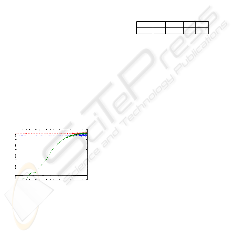
4.4.2 Performance Comparison

In this section we investigate the performance of the

adaptive strategy with respect to the reference strate-

gies in a non-stationary scenario. For this, we per-

formed some computer experiments for returns with

changing periodicity. As we did in the previous sec-

tions, we assumed for all strategies the parameter val-

ues q

min

= 0.1 and q

max

= 1.0 and for the strategy

MLS we used Eq. (11) to calculate the memory size,

M. For the strategy GACE, we used the parameter

values listed in Table 2 and the length of a chromo-

some in the range G

∈ (1,G

max

), with G

max

= 200.

We show in Fig. 4 (top) the evolution of budget for

different investment strategies, and (bottom) the cor-

responding periodicity of the returns, Eq.(4), both in

the course of time. Thus, the best strategy is the strat-

egy SW, following the strategy MLS; however, note

that both strategies have total and partial knowledge

about the dynamics of the returns, respectively. This

previous knowledge gives some advantage to these

strategies over the strategy GACE, which only needs

the speciﬁcation of G

max

. We note that the strategy

GACE evolves quite fast, yielding a set of investment

strategies with a clear tendency to lead more gains

than losses.

5 CONCLUSIONS

In this paper, we presented a simple investment model

and some investment strategies to control the propor-

tion of investment in cyclic changing environments.

The novelty of this paper is in the adaptive investment

strategy here proposed, called Genetic Algorithm for

Changing Environments (GACE), which is a new ap-

proach based on evolution for the correct mapping of

ICINCO 2008 - International Conference on Informatics in Control, Automation and Robotics

212

MLS

GACE

0 20000 40000 60000 80000 100000

100

Figure 4: (Top) Budget for different strategies and (bottom)

Periodicity of the returns, both in the course of time for RoI

with parameters T

max

= 100, t

max

= 10

and σ = 0.1.

investment proportionsto patterns that may be present

in the returns. We analyzed the performance of GACE

for different scenarios, and compared its performance

in the course of time against other strategies used here

as a reference. We showed that even though the strat-

egy GACE has no knowledge of the dynamics of the

returns, after a given number of time steps it may

lead to large gains, performing as well as other strate-

gies with some knowledge. This particularly is shown

for long-lasting periodicities, where an ever increas-

ing growth of budget was observed. Further work

includes the analysis of the performance of the strat-

egy GACE for real returns, and to compare the perfor-

mance of GACE against other approaches from Ma-

chine Learning.

ACKNOWLEDGEMENTS

We thank to Dr. Dagmar Monett for providing us the

program +CARPS. We also thank Frank Schweitzer

and H.-D. Burkhard for helpful advice.

REFERENCES

Dawid, H. (1999). Adaptive learning by genetic algorithms:

Analytical results and applications to economic mod-

els. Springer, Berlin.

Geibel, P. and Wysotzki, F. (2005). Risk-sensitive reinforce-

ment learning applied to control under constraints. J.

of Artif. Intell. Res., 24:81–108.

Grefenstette, J. J. (1992). Genetic algorithms for changing

environments. In Manner, R. and Manderick, B., ed-

itors, Parallel Problem Solving from Nature 2., pages

137–144. Elsevier, Amsterdam.

Harvey, I. (1992). The sage cross: The mechanics of recom-

bination for species with variable-length genotypes.

In Parallel Problem Solving from Nature, volume 2,

pages 269–278. Elsevier, Amsterdam.

Holland, J. H. (1975). Adaptation in Natural and Artiﬁcial

Systems. The University of Michigan Press.

Kahneman, D. and Tversky, A. (1979). Prospect theory of

decisions under risk. Econometrica, 47:263–291.

Kelly, J. L. (1956). A new interpretation of information rate.

AT&T Tech. J., 35:917–926.

LeBaron, B. (2001). Empirical regularities from interact-

ing long and short horizon investors in an agent-based

stock market. IEEE Transactions on Evolutionary

Computation, 5:442–455.

Magdon-Ismail, M., Nicholson, A., and Abu-Mostafa, Y.

(2001). Learning in the presence of noise. In Haykin,

S. and Kosko, B., editors, Intelligent Signal Process-

ing, pages 120–127. IEEE Press.

Michalewic¸z, Z. (1999). Genetic Algorithms + Data Struc-

tures = Evolution Programs. Springer, Berlin.

Monett, D. (2004). +CARPS: Conﬁguration of Metaheuris-

tics Based on Cooperative Agents. In Blum, C., Roli,

A., and Sampels, M., editors, Proc. of the 1

Int.

Workshop on Hybrid Metaheuristics, at the 16

Eu-

ropean Conference on Artiﬁcial Intelligence, (ECAI

’04), pages 115–125, Valencia, Spain. IOS Press.

Navarro, J. E. and Schweitzer, F. (2003). The investors

game: A model for coalition formation. In Czaja, L.,

editor, Proc. of the Workshop on Concurrency, Speci-

ﬁcation & Programming, CS&P ’03, volume 2, pages

369–381, Czarna, Poland. Warsaw University Press.

Navarro-Barrientos, J. E., Cantero-Alvarez, R., Rodrigues,

J. F. M., and Schweitzer, F. (2008). Investments in ran-

dom environments. Physica A, 387(8-9):2035–2046.

Richmond, P. (2001). Power law distributions and dynamic

behaviour of stock markets. The European Physical

Journal B, 20(4):523–526.

Schulenburg, S. and Ross, P. (2001). Strength and money:

An LCS approach to increasing returns. In Lecture

Notes in Computer Science, volume 1996, pages 114–

137. Springer.

Turing, G. (1960). An introduction to matched ﬁlters. IEEE

T. Inform. Theory., 6(3):311–329.

Yang, S. (2005). Experimental study on population-based

incremental learning algorithms for dynamics opti-

mization problems. Soft Computing, 9(11):815–834.

CONTROLLING INVESTMENT PROPORTION IN CYCLIC CHANGING ENVIRONMENTS

213