TEMPORAL SMOOTHING PARTICLE FILTER FOR VISION BASED

AUTONOMOUS MOBILE ROBOT LOCALIZATION

Walter Nistic

o and Matthias Hebbel

Robotics Research Institute (IRF), Technische Universit

at Dortmund, Otto-Hahn-Str. 8, Dortmund, Germany

Keywords:

Particle Filters, Vision Based Localization, Real Time Systems.

Abstract:

Particle ﬁlters based on the Sampling Importance Resampling (SIR) algorithm have been extensively and

successfully used in the ﬁeld of mobile robot localization, especially in the recent extensions (Mixture Monte

Carlo) which sample a percentage of particles directly from the sensor model. However, in the context of

vision based localization for mobile robots, the Markov assumption on which these methods rely is frequently

violated, due to “ghost percepts” and undetected collisions, and this can be troublesome especially when

working with small particle sets, due to limited computational resources and real-time constraints. In this

paper we present an extension of Monte Carlo localization which relaxes the Markov assumption by tracking

and smoothing the changes of the particles’ importance weights over time, and limits the speed at which the

samples are redistributed after a single resampling step. We present the results of experiments conducted on

vision based localization in an indoor environment for a legged-robot, in comparison with state of the art

approaches.

1 INTRODUCTION

Vision-based localization is becoming very popular

for autonomous mobile robots, and particle ﬁlters are

a successful technique to integrate visual data for lo-

calization. Due to size, cost and power consumption

limits, many robots use a camera as their only exte-

roceptive sensor; although range ﬁnders such as laser

scanners would provide more accurate measurements,

vision can often provide unique features such as land-

marks to speed up global localization.

1.1 The Platform

This work has been developed on the Sony Aibo

ERS-7 robot (Sony Corporation, 2004), which has

been one of the most popular complete standard plat-

forms adopted for robotic applications. The robot is

equipped with a 576MHz 64bit RISC CPU, 64MB of

main memory, and a low-power CMOS camera sen-

sor with a maximum resolution of 416X320 pixel.

The camera is mounted on the robot head, with 3 de-

grees of freedom in the neck; it is severely limited in

terms of resolution, ﬁeld of view (56.9

◦

horizontally),

and is affected by a signiﬁcant amount of noise. The

Aibo production has been recently discontinued by

Sony, but several new commercially available robotic

kits are being introduced, such as the humanoid robot

“Nao” from Aldebaran Robotics

, with similar char-

acteristics in terms of size and power, often equipped

with embedded RISC CPUs or PDAs and inexpensive

compact ﬂash cameras.

1.2 Related Work

Practical applications of particle ﬁlters for mobile

robot localization began with the introduction of the

Sampling Importance Resampling (SIR) ﬁlter pro-

posed in (Gordon et al., 1993), (Dellaert et al., 1999)

as an important extension of the Sequential Impor-

tance Sampling (SIS) ﬁlter (Geweke, 1989). The SIS

ﬁlter requires a huge number of particles to work,

since it does not make an efﬁcient use of them, as

the particle location is not inﬂuenced by sensor data

in any way; the resampling step introduced in the SIR

ﬁlter acts as a kind of “survival of the ﬁttest” strat-

egy that increases the particle density in the areas of

highest probability of the posterior distribution. How-

ever, in the context of mobile robot localization the

SIR ﬁlter suffers of two major problems: difﬁculty to

http://www.aldebaran-robotics.com/

Nisticò W. and Hebbel M. (2008).

TEMPORAL SMOOTHING PARTICLE FILTER FOR VISION BASED AUTONOMOUS MOBILE ROBOT LOCALIZATION.

In Proceedings of the Fifth International Conference on Informatics in Control, Automation and Robotics - RA, pages 93-100

DOI: 10.5220/0001497400930100

 SciTePress

recover in the “kidnapped robot” case (i.e. the robot

is moved by an external agent to a new location); and

ﬁlter degeneracy, where the ﬁlter performance starts

to drop instead of improving as the sensors become

“too” accurate, so that it becomes increasingly difﬁ-

cult to ﬁnd particles close enough to the peaks of the

likelihood function. Both problems can be (partially)

eased by increasing the number of particles used, but

this increases the computational cost; a much better

solution has been proposed in (Lenser and Veloso,

2000) which samples a certain percentage of parti-

cles directly from the sensor model (“Sensor Reset-

ting Localization” (SRL)), ensuring that no measure-

ment gets lost due to a lack of particles. A more

formal representation of the sensor resetting idea has

been described in (Thrun et al., 2001) with the “Mix-

ture Monte Carlo” (MMCL) algorithm, where a small

percentage of particles are sampled from the sensor

model and receive importance weights proportional to

the process model, thus (unlike SRL localization) the

belief converges to the true posterior for an inﬁnite

number of samples. In the context of vision based

localization on autonomous mobile robots, in (R

ofer

and J

ungel, 2003) the authors presented an approach

to deal with high levels of noise/uncertainty while us-

ing a small particle set (100 samples). Their approach

keeps track of the individual importance weights of

different landmark classes, and uses this information

to constrain the maximum change of likelihood of the

particle set in a single iteration of the algorithm, thus

easily rejecting outliers in the measured data. The

proposed approach is not formally correct, as we will

show, however it provides surprisingly good results in

practice and it is very popular on the Aibo platform,

thanks also to the availability of its source code

2 PARTICLE FILTERS

The Particle Filter (Fox et al., 2003) is a non-

parametric implementation of the general Bayes Filter

(Thrun et al., 2005). Given a time series of measure-

ments z

1:t

, control actions u

1:t

and an initial belief

p(x

), the Bayes Filter is a recursive algorithm that

calculates the belief or posterior bel(x

) at time t of

the state x

of a certain process, by integrating sensor

observations z

and control actions u

over the belief

of the state at time t − 1. The Bayes Filter is based on

the Markov assumption or complete state assumption

which postulates the conditional independence of past

and future data given the current state x

. This can

be expressed in terms of conditional independence as

http://www.germanteam.org/GT2005.zip

follows:

p(z

, z

1:t

, u

1:t

) = p(z

)

p(x

t−1

, z

1:t−1

, u

1:t

) = p(x

, x

t−1

)

(1)

A Particle Filter represents an approximation of the

posterior bel(x

) in the form of a set of samples ran-

domly drawn from the posterior itself; such a repre-

sentation has the advantage, compared to closed form

solutions of the Bayes Filter such as the Kalman Fil-

ter (Kalman, 1960), of being able to represent a broad

range of distributions and model non-linear processes,

whereas parametric representations are usually con-

strained to simple functions such as Gaussians. In

the context of robot localization and object tracking,

particle ﬁlters are often referred to as Monte Carlo

Localization. Given a set of N samples or parti-

cles χ

:= x

, x

, . . . , x

, at time t each particle

represents an hypothesis of the state of the observed

system; in case of robot localization, the state space

is usually represented by the (x, y) cartesian coordi-

nates in the plane, and the heading θ. Obviously, the

higher the number of samples N , the better the ap-

proximation, however (Fox, 2003) has shown how to

dynamically adjust N . In this work we do not con-

sider dynamic adjustments in the number of samples

used, since we are interested in keeping the run-time

of the algorithm approximately constant, due to the

real-time constraints. An estimate of p(x

, x

t−1

)

Algorithm 1 : SIR Particle Filter.

Require: particle distribution χ

t−1

, control action

, measurement observation z

for i = 1 to N do

1. Process update: update the particles’ state

as the result of the control action u

: x

∼

p(x

, x

t−1

)

2. Measurement update: calculate the particle

importance factors w

= p(z

) from the latest

observation

Add



, w



to the temporary set χ

end for

3. Resampling: create χ

from χ

by drawing the

particles x

in number proportional to their impor-

tance w

. All the importance factors w

in χ

are

reset to 1.

is called Process Model, while p(z

) is known as

Sensor Model. χ

before the measurement update

step is a sampled representation of the prior distri-

bution bel(x

). If we omit the Resampling step in Al-

gorithm 1we obtain the SIS ﬁlter. Under the Markov

assumption, current measurements are statistically in-

dependent from past measurements, as such the im-

portance factors during the Measurement update step

ICINCO 2008 - International Conference on Informatics in Control, Automation and Robotics

can be calculated as:

= p(z

) · w

t−1

(2)

The SIS ﬁlter for localization generally performs

poorly, in fact since the importance weights are up-

dated multiplicatively, a single percept is sufﬁcient to

set the importance of a given particle close to zero. It

has been formally demonstrated that the variance of

the importance weights in the SIS ﬁlter can only in-

crease (stochastically) over time (Doucet et al., 2000).

The SIR ﬁlter performs much better, because after the

resampling step, the particles of low importance are

discarded while the particles of high importance are

replicated and all the importance weights are reset to

1, i. e. all particles carry the same importance. Con-

sequently the distribution approximates the true pos-

terior bel(x

) = ηp(z

)bel(x

2.1 Sampling from Observations: The

Kidnapped Robot Problem

The situation when a mobile robot is physically

moved (“teleported”) by an external agent in a new lo-

cation is known as the “Kidnapped Robot” problem.

This situation is challenging because the robot has no

information about such external action and its sensor

and control data is not in accordance with the new

state. The SIR ﬁlter as it has been presented has seri-

ous problems dealing with this situation, because it is

unlikely to ﬁnd a particle in the proximity of the loca-

tion where the robot has been teleported, due to the ef-

fect of resampling which tends to concentrate the par-

ticle distribution in the area of high likelihood of the

posterior at time t − 1, which in this case corresponds

to the robot’s location prior to the teleporting action.

An efﬁcient solution to such problem is to reverse the

Monte Carlo process (“Dual Monte Carlo”) by draw-

ing a certain percentage of the samples directly from

the measurement model instead of the prior belief dis-

tribution :

∼ p(z

) (3)

and calculate the importance weights from the prior

distribution (integrating the process model):

p(x

, x

t−1

)bel(x

t−1

)dx

t−1

(4)

Dual Monte Carlo performs better than normal MCL

with very precise sensors, and can quickly recover

in case the robot is teleported, since the samples are

drawn directly from the last observations. Conversely,

it is extremely sensitive in case of high sensor noise

and performs poorly especially with ghost percepts;

for these reasons, Mixture Monte Carlo uses a small

percentage of samples which are updated using the

Dual MCL approach, and the rest are following the

normal MCL algorithm, thus combining the beneﬁts

of both approaches. The main implementation prob-

lems of the Dual MCL approach is that it is often dif-

ﬁcult to sample from the observation model (Equation

3), when such model does not have a closed form, and

it is both difﬁcult and computationally expensive to

calculate the importance weights from the prior dis-

tribution (Equation 4).

3 TEMPORAL SMOOTHING

PARTICLE FILTER

Particle ﬁlters can generally deal efﬁciently with sen-

sor noise, provided that there is a sufﬁcient amount

of particles (most authors suggest to use at least 1000

particles) and that the measurement model is accurate

enough. However a limit of this approach is that in

practice the Markov assumption can often be violated:

unmodeled dynamics in the environment, such as the

presence of other mobile agents, “ghost” percepts (for

example, echoes in sonar data, or incorrectly classi-

ﬁed objects in a vision system), inaccuracies in the

probabilistic sensor and process model (slippage, col-

lisions), approximation errors due to the sampled rep-

resentation, etc.

3.1 Sensor Smoothing

In (R

ofer and J

ungel, 2003) the authors proposed an

approach which can deal with highly noisy visual

measurements while using a sample set of just 100

particles, which can then be executed in real-time on

severely constrained (in terms of processing power)

mobile robots. The idea is to limit the effect of a sin-

gle measurement (which might be an outlier) on the

particle population; this is achieved by constraining

the measured importance weight ¯w

for a given parti-

cle at time t to differ at most by a ﬁxed ∆ from the

value that the particle had at time t − 1.







t−1

+ ∆

) if( ¯w

> w

t−1

+ ∆

)

t−1

− ∆

) if( ¯w

< w

t−1

− ∆

)

¯w

else

(∆

= 0.01, ∆

= 0.005)

(5)

The visual features used for localization are separated

in a set of different percept classes (ﬁeld lines, bor-

ders and goals are the recognized objects in (R

ofer

and J

ungel, 2003)), the perceived measurements of

different classes are assumed to be statistically inde-

pendent, and each particle carries a different impor-

tance weight per percept class. Consequently, the im-

TEMPORAL SMOOTHING PARTICLE FILTER FOR VISION BASED AUTONOMOUS MOBILE ROBOT

LOCALIZATION

portance weight of a particle is calculated as the prod-

uct of the weights associated to each percept class.

From a theoretical point of view, the smoothing per-

formed in Equation 5 is a violation of the Markov as-

sumption, in fact past and current measurements for

objects in the same class are correlated by this up-

date method. This can be seen as an incremental es-

timate of the importance weight of a given particle

with respect to a series of measurements of a certain

object, rather than considering each measurement in-

dependently. For this reason, this method can easily

ﬁlter noise in the measurements, as well as limit the

effects of outliers, since it takes a series of consis-

tent measurements to affect signiﬁcantly the distribu-

tion. However, this approach as presented in (R

ofer

and J

ungel, 2003) has some problems:

1. having ∆

6= ∆

introduces an unnecessary

bias in the importance weights;

2. since measurements relative to different objects

are put in the same class, and the particles keep

their “memory” indeﬁnitely, this mechanism in-

correctly correlates measurements which should

be independent.

While ﬁxing the ﬁrst problem is trivial, the same is not

true about the second; the correct solution would be

to assign a different percept class to each perceived

object, so that they can be treated as statistically in-

dependent. This however is not always possible, be-

cause in some cases the robot is observing different

objects which are undistinguishable, like walls in vi-

sion based localization, or range measurements with

laser scanners. Thus, here we introduce an “aging

law” which fades out the memory of past measure-

ments in the importance weights, thus reducing the in-

correct correlations among percepts of the same class.

This corresponds to an assumption of temporal co-

herence of a series of measurements, i. e. we expect

“bursts” of measurements relative to a certain object

to appear for a short time. So, if we deﬁne a set Γ of

percept classes, let w

i,j

be the importance weight for

the percept class j ∈ Γ relative to the i-th particle at

time t, α

∈ [0..1] an aging factor for class j, then the

result of the aging process ˆw

i,j

can be calculated as:

ˆw

i,j

= w

i,j

+ (1 − w

i,j

) · α

(6)

This function asymptotically fades an importance fac-

tor toward 1 (i. e. that percept class does not affect the

global importance factor of that particle), with a speed

controlled by the parameter α

, which can be set ac-

cording to the frequency of independent observations

of a given percept class. For α tending to 0, the par-

ticles keep “memory” of old percepts for a long time,

while for α tending to 1 the particle weights are re-

set in each iteration like in the SIR ﬁlter. This is also

beneﬁcial in case a series of past measurements for a

given class resulted in a very low weight, which with-

out aging would affect negatively the global weight

of the particle, regardless of the values of the other

percept classes. Finally, after the aging step (Equa-

tion 6), given a ¯w

i,j

calculated from the measurement

model, we can apply the temporal smoothing step:

i,j







( ˆw

i,j

t−1

+ ∆

) if( ¯w

i,j

> ˆw

i,j

t−1

+ ∆

)

( ˆw

i,j

t−1

− ∆

) if( ¯w

i,j

< ˆw

i,j

t−1

− ∆

)

¯w

i,j

else

j∈Γ

i,j

(7)

3.2 “lazy” Resampling

The main problem of the approach described in

ofer and J

ungel, 2003) is the resampling step: par-

ticles are copied in the new distribution χ with a fre-

quency proportional to their importance weight w

as in the Step 3 of Algorithm 1, but the weights w

i,j

are not reset to 1 afterward, this because otherwise it

would not be possible to use them to ﬁlter the mea-

surements at the following iterations of the algorithm.

So, supposing that a particle with importance w

copied n

> 1 times in the target distribution χ, the

probability density in that location will increase by a

factor of n

. Consequently, after the resampling step

the particle distribution does not approximate the true

posterior anymore: the probability density will artiﬁ-

cially increase in areas of high likelihood, while it will

further decrease in areas of low likelihood. The re-

sult is that this ﬁlter converges very quickly and tends

to focus most of the particles around the main peak

of the probability distribution; in practice the ﬁlter

works very well as long as the noise can be ﬁltered

by its sensor smoothing mechanism, but when there

is a high level of ambiguity in the sensor data, for ex-

ample if no unique landmark is observed in a long

time, then the particles will start to quickly oscillate

among different peaks of the true posterior distribu-

tion, rather than assume a multi-modal distribution.

This problem can be ﬁxed however, if we know the

number of times n

that a certain particle i has been

copied. This can be used to normalize the weights in

the target distribution, so that it again approximates

the posterior:

˜w

⇒

j∈Γ

i,j

j∈Γ

⇒

j∈Γ

i,j

; c = kΓk

(8)

ICINCO 2008 - International Conference on Informatics in Control, Automation and Robotics

where, given n

and c (the number of percept classes)

we can normalize the global weight of the particle ˜w

dividing its importance weights by the coefﬁcient ν

As the basis for our new resampling algorithm, we

use the low variance sampler (Thrun et al., 2005).

The low variance sampler has several advantages over

Algorithm 2 : Low Variance Sampling.

Require: proposal particle distribution ¯χ

, impor-

tance weights W

, number of particles N

= ∅

r = rand(0; N

−1

)

c = w

i = 1

for m = 1 to N do

U = r + (m − 1) · N

−1

while U > c do

i = i + 1

c = c + w

end while

add x

to χ

end for

return target distribution χ

the independent random sampler described in the ba-

sic SIR ﬁlter algorithm: it has O(N ) complexity (in-

stead of O(N log(N ))), it guarantees that if all parti-

cles have the same importance, χ

is the same as ¯χ

and most importantly for us, it covers the set of sam-

ples systematically, making it much easier to track the

values n

to use for normalization. At this point, we

can introduce a new technique, that here we will call

“lazy resampling”, to enforce temporal coherence in

the particle distribution: we can clip the number of

new samples in the target distribution χ which can be

generated from a single particle in the proposal dis-

tribution ¯χ to be at most a chosen ¯n

max

∈ [1..N ].

The idea is to reduce the effect of a single resampling

step on the particle distribution: if a robot is well lo-

calized and it is not teleported, we would expect that

the peaks of the posterior distribution at time t are

close to the position they had at time t − 1, factoring

in the odometry data in the process update step. Es-

pecially when drawing some samples from the mea-

surement model, as in the Sensor Resetting / Mixture

Monte Carlo approaches described, a few bad mea-

surements would move many particles away from the

area of high likelihood, degrading the performance of

the ﬁlter; by setting a limit to the number of times

that a single particle can be copied as a consequence

of resampling, we are reducing the effects of outliers

on the particle distribution. The downside is that, in

case the robot is really teleported, our ﬁlter would be

slower in relocating most of the particles in the new

area of high likelihood: the robot would still relocate

its estimate quickly, because of the update in the par-

ticle importance weights, but there would be initially

less resolution in the area where the robot has been

teleported. Thus, it is necessary to set a value of ¯n

max

as a compromise dependent on the frequency of robot

teleports and the amount of sensor noise and ambigu-

ity. For ¯n

max

= 1, a particle in ¯χ is copied unaltered

in χ, as such the SIS ﬁlter can be seen as a special case

of our lazy resampling; at the other end of the spec-

trum, setting ¯n

max

= N results in no limitations in

the effects of resampling, so our ﬁlter behaves exactly

like a SIR ﬁlter. Algorithm 3 describes a possible im-

plementation, r is used to calculate how many times a

certain particle should be copied in the target distribu-

tion based on its importance weight; such number is

clipped to a maximum resample limit of ¯n

max

. Par-

ticles of low weight (n < 1) are copied in the target

distribution starting from the end of the list (indexed

by j), so that they can be overwritten by the more im-

portant particles, which are copied starting from the

beginning of the list (indexed by i).

Algorithm 3 : “Lazy” Resampling.

Require: proposal particle distribution ¯χ

, impor-

tance weights W

, number of particles N , resample

limit ¯n

max

= ∅

i = 1

j = N

r =

for m = 1 to N do

n = min(br · w

c; ¯n

max

)

if n > 0 then

normalize ˜w

for z = 1 to n do

add x

, ˜w

in position i

i = i + 1

end for

else

if j > i then

add x

, w

in position j

j = j − 1

end if

end for

return target distribution

TEMPORAL SMOOTHING PARTICLE FILTER FOR VISION BASED AUTONOMOUS MOBILE ROBOT

LOCALIZATION

4 EXPERIMENTS AND RESULTS

In the following experiments, we will evaluate the

performance of our new approach (from now on

referred to as Temporal Smoothing Monte Carlo

“TSMCL”) which uses our sensor smoothing with ag-

ing (Equations 6,7) and the lazy resampling strategy

described in Algorithm 3. We compare it with a SIR

ﬁlter with Sensor Resetting, and the approach de-

scribed in (R

ofer and J

ungel, 2003) (here for conve-

nience referred to as Sensor Smoothing Monte Carlo

“SSMCL”).

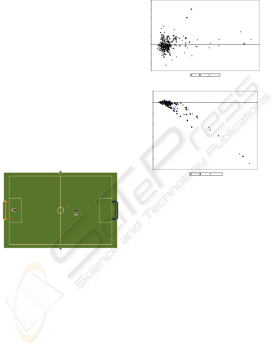
4.1 Test Environment

The robot is placed in a soccer ﬁeld whose size is

6m×4m, where it can recognize 4 unique landmarks:

2 goals (1 yellow, 1 blue) and 2 cylindrical beacons

(yellow on blue, and blue on yellow). The position

of the landmarks on the map is known to the robot.

Additionally, the robot can recognize non unique fea-

tures such as the white lines on the ﬁeld, and the inter-

sections where the lines meet (see Figure 1). Since the

Figure 1: Test environment: a yellow and a blue goal, two

colored beacons (on the middle line), two robots and an or-

ange ball.

environment is color coded, the vision system, simi-

lar to the approach described in (Nistic

o and R

ofer,

2006), uses color based image segmentation. The vi-

sion and localization systems run at 30 frames per sec-

ond.

As can be seen in Figure 2, the measurement error

is high (especially the measured distance error grows

almost exponentially with the distance to the observed

object), due to the low resolution of the camera and

the fact that the camera pose in space can only be

roughly estimated. In fact the camera is mounted on

the head of the robot, it has 3 degrees of freedom and

due to the narrow ﬁeld of view, it has to constantly

scan around at high angular velocity. Moreover, the

-30

-20

-10

0 2000 4000 6000 8000 10000 12000 14000 16000

Beacons Blue Goal Yellow Goal

(a) Bearing Error

-12000

-10000

-8000

-6000

-4000

-2000

2000

0 2000 4000 6000 8000 10000 12000 14000 16000

Beacons Blue Goal Yellow Goal

(b) Distance Error

Figure 2: Landmark Measurement error. The bearing (de-

grees) and distance (mm) errors are plotted as a function of

the perceived distance.

height of the neck on which the camera is mounted is

not constant since the robot uses legged locomotion,

and it can only be approximately estimated through

kinematic calculations from the servos’ encoders in

the robot legs. For these reasons our sensor model

calculates the measurement error in terms of hori-

zontal angle (bearing) and vertical angle (depression)

to the observed object. This has the advantage that,

while the distance error grows more than linearly with

the real distance to the object, the vertical angle er-

ror variance is approximately constant. We assume

the horizontal and vertical angle error components to

be independent, and use gaussian likelihood functions

to model each component, with different constants

horizontal

, σ

vertical

, j ∈ Γ for each percept class.

Field lines and their intersections (crossings) due to

their small size can only be recognized reliably up to

a maximum distance of approximately 800mm; for

these non-unique features we adopt a closest point

matching model (with pre-computed lookup tables)

as described in (R

ofer and J

ungel, 2003). Due to the

different measurement errors (see Table 1) and fre-

quency of detection, we distinguish our percepts in 3

different classes: Γ = {Beacons, Goals, Lines}.

ICINCO 2008 - International Conference on Informatics in Control, Automation and Robotics

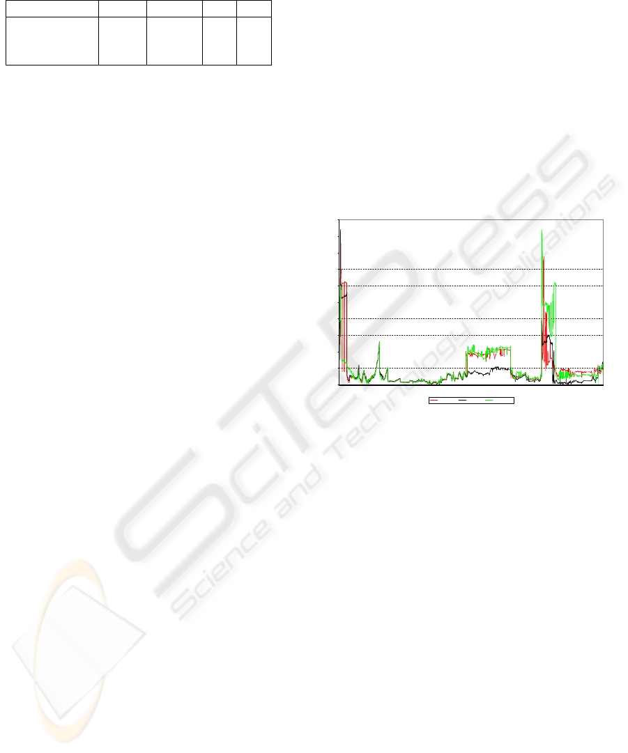
Table 1: Measurement error. ρ represents the distance error,

in expressed in mm; α the bearing error, in deg..

Percept Class µ

Beacons 162.7 178.5 3.2 3.1

Goals 708.5 1294.6 4.6 4.8

Lines 122.6 215.8 3.1 3.5

All three localization algorithms use overall 100

particles, draw a small percentage of them directly

from observations, and are executed in parallel in real-

time on our test platform. The locations for such sam-

ples are calculated from landmarks via triangulation

or using two bearings and two distances; for this pur-

pose, the location of seen landmarks is retained for

5 seconds and updated using odometry information.

Additionally, line crossings are classiﬁed as T-shaped

or L-shaped, and samples are drawn from all possi-

ble locations which match the seen shape (8 at most,

for L-shaped crossings, hence we use a mixture with

8% of particles drawn from observations), and two

further possible poses are found if the center circle is

seen. To provide ground truth to evaluate the localiza-

tion performance, we use an external vision system

based on a ceiling-mounted camera which is able to

track the robot position at 25 frames per second with

a maximum error of 40mm (position) and 2

◦

degrees

(heading). The process model updates the particle

positions based on odometry data which is provided

by the robot’s motion module; the odometry error is

modeled as a bi-dimensional gaussian with the ma-

jor axis parallel to the direction of movement, and an

independent gaussian represents the heading error.

4.2 Experiments

In the static localization case, with the robot hav-

ing unlimited time to reach a speciﬁed position on

the ﬁeld, all three approaches are able to localize the

robot with a position error below 7 cm and heading

error below 3 degrees, and in this situation it is not

possible to make an analysis of the relative perfor-

mance, due to measurement errors in the ceiling cam-

era system providing ground truth and the ﬂuctuations

derived from the randomized nature of the localiza-

tion algorithms employed. So in the following exper-

iments, we will analyze the accuracy of localization

while the robot runs around the ﬁeld: in the ﬁrst half

of each experiment the robot will be allowed to look

around to see unique landmarks, in the second half it

will be chasing a ball looking only at it, hence see-

ing landmarks only occasionally, having to rely on

non-unique features such as lines and crossings for

localization. In the ﬁrst experiment, we want to il-

lustrate the effects of our lazy resampling, by com-

paring the performance of our algorithm for different

values of the resample limit ¯n

max

: 8 (the experimen-

tally derived optimum for our application), 15 and

30 (for all practical purposes, equivalent to “unlim-

ited”, given a set of 100 particles). As can be seen

in Figure 3, all three versions localize about at the

same time (≈ 180 frames or 6 seconds), then they

perform equally well, as long as the robot receives

reasonably good percepts. However, in the situations

where the robot looks only at the ball for a long time,

the version with ¯n

max

= 8 performs much better, be-

ing more effective in smoothing the noise and resolv-

ing ambiguities by keeping more particles in the areas

where the robot was previously localized. In the sec-

500

1000

1500

2000

2500

3000

3500

4000

4500

5000

1 206 411 616 821 1026 1231 1436 1641 1846 2051 2256 2461 2666 2871 3076 3281 3486 3691 3896 4101 4306 4511 4716 4921 5126 5331 5536 5741 5946

15 Particles 8 Particles 30 Particles

Figure 3: Resample limit comparison (Test 1). x-axis: time

(frames); y-axis: position error. At frames 2900-3950 and

4700-5100 the scarcity of unique features and the odometry

errors make the localization jump to a wrong location.

ond experiment, we compare our TSMCL algorithm

with ¯n

max

= 8 to the state of the art approaches. In

the ﬁrst half of the experiment, all systems perform

equally well, with TSMCL and SIR nearly identical

and SSMCL slightly worse but within the limits due

to random factors. When the robot starts to chase

the ball however (after frame 3000), SIR and SSMCL

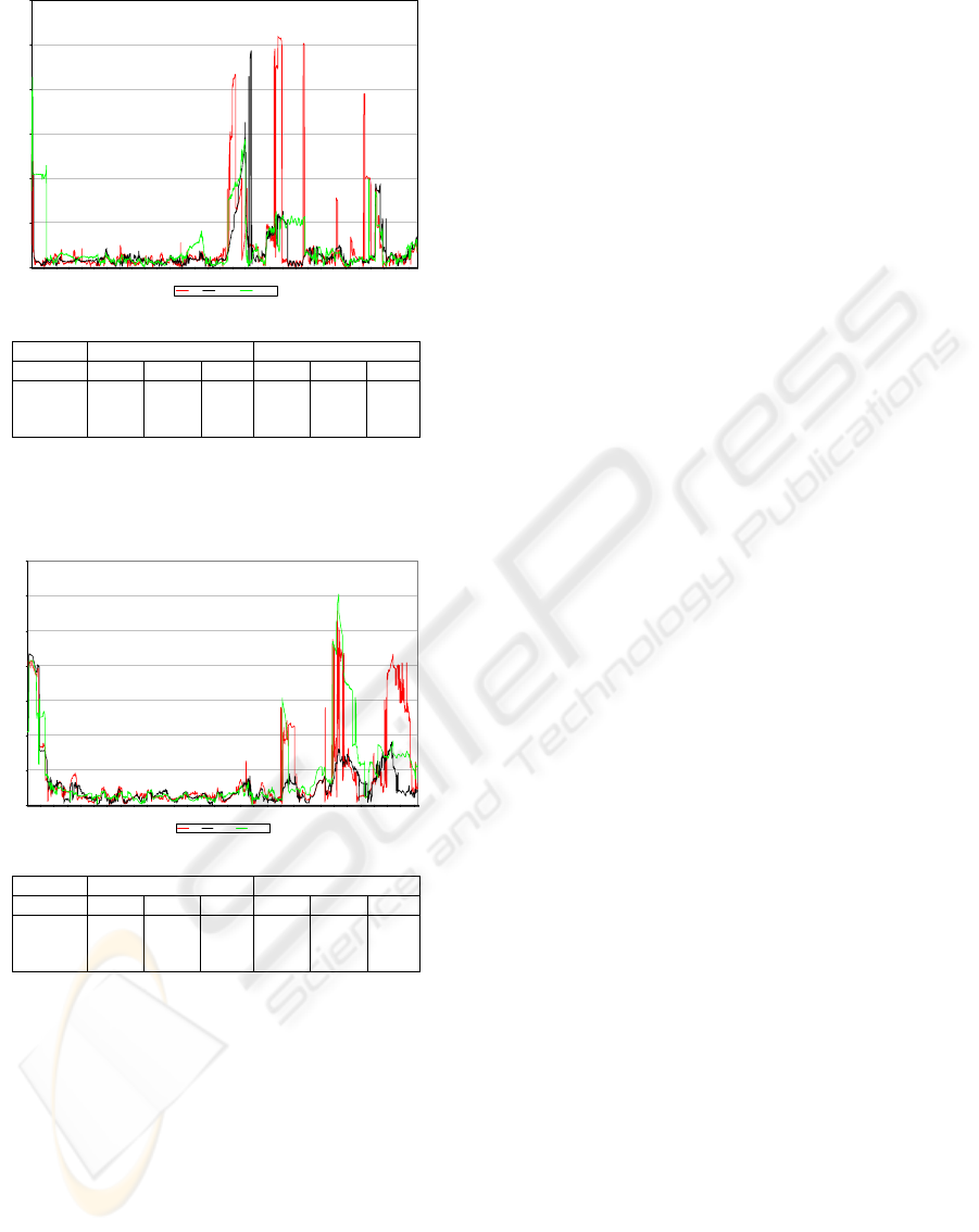
start to oscillate much more (Figure 4). Our third test

is similar to the second, but it represents a worse sce-

nario since this time the beacons (which are the best

landmark, in terms of measurement error and ease of

detection) are removed. The results presented in Fig-

ure 5 show our approach clearly outperforming the

others. The run-time of all 3 algorithms is 3−5ms per

frame, depending on the number and type of percepts

seen. We could not measure signiﬁcant differences in

the time taken to globally localize and recover from

kidnapping (2 − 6s in all cases).

TEMPORAL SMOOTHING PARTICLE FILTER FOR VISION BASED AUTONOMOUS MOBILE ROBOT

LOCALIZATION

1000

2000

3000

4000

5000

6000

1 228 455 682 909 1136 1363 1590 1817 2044 2271 2498 2725 2952 3179 3406 3633 3860 4087 4314 4541 4768 4995 5222 5449 5676 5903 6130

SIR TSMCL SSMCL

(a)

First Half Overall

µ σ max µ σ max

TSMCL 144.8 62.8 430 323.6 503.0 4864

SSMCL 201.9 130.3 813 444.1 553.1 2875

SIR 146.2 76.1 548 436.7 897.1 5195

(b)

Figure 4: Localization algorithm comparison (Test 2). x-

axis: time (frames); y-axis: position error.

1000

2000

3000

4000

5000

6000

7000

1 197 393 589 785 981 1177 1373 1569 1765 1961 2157 2353 2549 2745 2941 3137 3333 3529 3725 3921 4117 4313 4509 4705 4901 5097 5293 5489 5685

SIR TSMCL SSMCL

(a)

First Half Overall

µ σ max µ σ max

TSMCL 277.5 160.1 847 432.7 355.0 1811

SSMCL 276.3 128.6 867 745.8 998.1 6051

SIR 294.2 169.0 1261 706.9 993.7 5567

(b)

Figure 5: Localization algorithm comparison (Test 3). x-

axis: time (frames); y-axis: position error.

5 FUTURE WORK

We have presented an extension of Monte Carlo

Localization which exploits temporal smoothing to

improve localization accuracy in presence of high

amounts of noise and sensor ambiguity. In the fu-

ture we would like to apply our algorithm to multi-

object tracking, where its use of temporal coherence

could allow it to “keep memory” of multiple modes

in the distribution more effectively than normal parti-

cle ﬁlters, making it a good candidate to compete with

banks of multiple ﬁlters with degrees of association.

REFERENCES

Dellaert, F., Fox, D., Burgard, W., and Thrun, S. (1999).

Monte carlo localization for mobile robots. In IEEE

International Conference on Robotics and Automation

(ICRA99).

Doucet, A., Godsill, S., and Andrieu, C. (2000). On se-

quential monte carlo sampling methods for bayesian

ﬁltering. Statistics and Computing, 10:197–208.

Fox, D. (2003). Adapting the sample size in particle ﬁlters

through kld-sampling. I. J. Robotic Res., 22(12):985–

1004.

Fox, D., Hightower, J., Liao, L., Schulz, D., and Borriello,

G. (2003). Bayesian Filtering for Location Estimation.

PERVASIVE computing, pages 10–19.

Geweke, J. (1989). Bayesian inference in econometric

models using monte carlo integration. Econometrica,

57(6):1317–39.

Gordon, N. J., Salmond, D. J., and Smith, A. F. M. (1993).

Novel approach to nonlinear/non-gaussian bayesian

state estimation. Radar and Signal Processing, IEE

Proceedings F, 140(2):107–113.

Kalman, R. E. (1960). A new approach to linear ﬁltering

and prediction problems. Transactions of the ASME -

Journal of Basic Engineering, 82:35–45.

Lenser, S. and Veloso, M. (2000). Sensor resetting local-

ization for poorly modelled mobile robots. In Pro-

ceedings of the IEEE International Conference on

Robotics and Automation, 2000.

Nistic

o, W. and R

ofer, T. (2006). Improving percept reli-

ability in the sony four-legged league. In RoboCup

2005: Robot Soccer World Cup IX, Lecture Notes in

Artiﬁcial Intelligence, pages 545–552. Springer.

ofer, T. and J

ungel, M. (2003). Vision-Based Fast and

Reactive Monte-Carlo Localization. In Proceedings of

the 2003 IEEE International Conference on Robotics

and Automation, ICRA 2003, September 14-19, 2003,

Taipei, Taiwan, pages 856–861. IEEE.

Sony Corporation (2004). OPEN-R SDK Model Informa-

tion for ERS-7. Sony Corporation.

Thrun, S., Burgard, W., and Fox, D. (2005). Probabilistic

Robotics. Number ISBN 0-262-20162-3. MIT Press.

Thrun, S., Fox, D., Burgard, W., and Dellaert, F. (2001).

Robust monte carlo localization for mobile robots. Ar-

tiﬁcial Intelligence, 128(1-2):99–141.

ICINCO 2008 - International Conference on Informatics in Control, Automation and Robotics

100