
OBDD COMPRESSION OF NUMERICAL CONTROLLERS
Giuseppe Della Penna, Nadia Lauri, Daniele Magazzeni
Computer Science Department,University of L’Aquila, L’Aquila, Italy
Benedetto Intrigila
Department of Mathematics, University of Roma ”Tor Vergata”, Roma, Italy
Keywords:
Numerical Controllers, Compression Techniques, Ordered Binary Decision Diagrams.
Abstract:
In the last years, the use of control systems has become very common, especially in the embedded systems
contained in a growing number of everyday products. Therefore, the problem of the automatic synthesis of
control systems is extremely important. However, most of the current techniques for the automatic generation
of controllers, such as cell-to-cell mapping, dynamic programming, set oriented approach or model checking,
typically generate numerical controllers that cannot be embedded in limited hardware devices due to their
size.
A possible solution to this problem is to compress the controller. However, most of the common lossless
compression algorithms, such as LZ77, would decrease the controller performances due to their decompression
overhead.
In this paper we propose a new, completely automatic OBDD-based compression technique that is capable of
reducing the size of any numerical controller up to a space savings of 90% without any noticeable decrease in
the controller performances.
1 INTRODUCTION
Control systems (or, shortly, controllers) are small
hardware/software components that control the be-
havior of larger systems, the plants. A controller con-
tinuously looks at the plant state variables and possi-
bly adjusts some of its control variables to keep the
system in the setpoint, which usually represents its
correct behavior.
In the last years, the use of controllers has become
very common in robotics, critical systems and, in gen-
eral, in the embedded systems contained in a growing
number of everyday products. Therefore, the prob-
lem of the automatic synthesis of control systems is
extremely important.
To this aim, several techniques have been devel-
oped, based on a more or less systematic exploration
of the plant state space. One can mention, among oth-
ers, cell-to-cell mapping techniques (Leu and Kim,
1998), dynamic programming (Kreisselmeier and
Birkholzer, 1994) and set oriented approach (Gr¨une
and Junge, 2005). Recently, model checking tech-
niques have also been applied (Della Penna et al.,
2006; Della Penna et al., 2007b) in the field of au-
tomatic controller generation.
The controllers generated using all these tech-
niques are typically numerical controllers, i.e. tables
indexed by the plant states, whose entries are com-
mands for the plant. These commands are used to
set the control variables in order to reach the setpoint
from the correspondingstates. Namely, when the con-
troller reads a state from the plant, it looks up the ac-
tion described in the associated table entry and sends
it to the plant.
However, a main problem of this kind of con-
trollers is the size of the table, which for complex sys-
tems may contain millions of entries, since it should
be embedded in the control system hardware that is
usually very limited.
A possible solution to these problems is to derive,
from the huge numerical information contained in the
table, a small fuzzy control system. This solution is
natural since fuzzy rules are very flexible and can
be adapted to cope with any kind of system. More-
43
Della Penna G., Lauri N., Magazzeni D. and Intrigila B. (2008).
OBDD COMPRESSION OF NUMERICAL CONTROLLERS.
In Proceedings of the Fifth International Conference on Informatics in Control, Automation and Robotics - ICSO, pages 43-50
DOI: 10.5220/0001497900430050
Copyright
c
SciTePress

over, there are a number of well-established tech-
niques to guide the choice of fuzzy rules by statisti-
cal considerations, such as in Kosko space clustering
method (Kosko, 1992), by abstracting them from a
neural network (Sekine et al., 1995), by clustering the
trajectories obtained from the cell mapping dynam-
ics (Leu and Kim, 1998) and finally by using genetic
algorithms (Della Penna et al., 2007a).
However, two considerations are to be made with
respect to this approach. First, the detection of the
fuzzy rules requires (at least) a tuning phase which
is not completely automatic but involves some human
intervention. Second, the fuzzy rules appear not to
be suitable when a very high degree of precision is
needed. This is the case, e.g., of the truck and trailer
parking problem when obstacles are to be avoided in
the parking lot (Della Penna et al., 2006). In this case,
when the truck is near to an obstacle, only a very pre-
cise manoeuvre can park it, without hitting the obsta-
cle. So, to achieve the required precision, an exceed-
ing number of fuzzy rules would be necessary.
Therefore, it seems reasonable to pursue another
possible approach, that is to directly compress the
control table. By this we mean data compression
in the usual sense of reduction of the number of bits
needed to represent the controller table in the com-
puter RAM memory (Cover and Thomas, 2006; Nel-
son and Gailly, 1995).
Observe, however, that in this case the compres-
sion algorithm should be constrained as follows:
1. the logical content of the table, that is the rela-
tion between the states and the correspondingcon-
trol actions, must be preserved without any loss of
information (i.e., we need some kind of lossless
compression algorithm);
2. the access time to the table must be comparable
with the one obtained with a direct representation
of the table in the computer memory (i.e., the de-
compression overhead must be minimal).
Consider as an example the straightforward idea
of directly compressing the table by mean of (some
variant of) the well known Lempel-Zivalgorithm (Ziv
and Lempel, 1977). Since this is a lossless compres-
sion, the first requirement above is fulfilled, but not
the second one, since the access time to the table
would be linear in the uncompressed size of the table
itself (Nelson and Gailly, 1995).
Since all the common compression algorithms
have similar problemswhen applied to controllers, we
decided to develop a new ad-hoc compression algo-
rithm based on the well known Ordered Binary Deci-
sion Diagrams (OBDDs) (Bryant, 1986).
Decision diagrams as well as decision trees are of
wide use in data manipulation as well as in data min-
ing (Hand et al., 2001). Indeed, our choice of OB-
DDs was motivated by their capability of compress-
ing large state spaces, that is at the hearth of symbolic
model checking and of its great achievements (Burch
et al., 1992; Clarke et al., 1999). Our hypothesis has
been that this capability is transferrable to the com-
pression of the controller table which is, in a sense,
an augmented state space representation.
Our experimental results show that this is indeed
the case. For very large tables we obtain a quite good
compression ratio (around 10:1). Moreover, not only
the access time is good, but it is often even better than
the one obtained by a direct representation of the ta-
ble in memory. This phenomenon is due to the fact
that, unless we accept a very sparse table, with huge
waste of space, we need to represent the controller
using some kind of open addressing table accessed
through a hash function, with a consequent worsen-
ing of the access time (Cormen et al., 2001).
A final but very important point to be stressed is
that the implemented compression algorithm, which
transforms the controller table in an OBDD, operates
in a completely automatic way. The only parameter
the user should set is the BDD variable reordering
method (see Section 4), which can effect the com-
pression ratio. After that, the compression operates in
a “zip”-like fashion. However, the best setting of the
above parameter can also be discovered by the algo-
rithm by trying all the possible reorderings, thus mak-
ing the compression process completely automatic.
Finally, a further automatic step can also be applied
to transform the OBDD into C-code that can be in-
corporated in any C-program.
The paper is organized as follows: in Section 2
we give a description of OBDDs and in Section 3
we show how we use them to encode numerical con-
trollers. In Section 4 we present our experimental re-
sults and Section 5 concludes the paper.
2 ORDERED BINARY DECISION
DIAGRAMS
A Binary Decision Diagram (BDD) is a data structure
used to represent a boolean function (Bryant, 1986).
Indeed, any boolean function f can be represented
as a binary tree having two kind of leaf values: F
(boolean false) or T (boolean true). Each node of
the tree (decision node) is labeled by a variable of the
formula f. The two edges outgoing a decision node
represent an assignment of the corresponding variable
to false or true, respectively. Therefore, a path from
the BDD root to one of its leaves represents a (pos-
sibly partial) variable assignment for f , and the cor-
ICINCO 2008 - International Conference on Informatics in Control, Automation and Robotics
44
responding leaf value is the value of f for the given
assignment.
An advantage of BDDs is that many logical op-
erations, like conjunction, disjunction, negation or
abstraction can be implemented by polynomial-time
graph manipulation algorithms. Indeed, BDDs are ex-
tensively used in the software tools, e.g., to synthesize
circuits or to perform formal verifications.
If variables appear in the same order on all paths
(or, in other words, if all the nodes on the same tree
level refer to the same variable) the BDD is called
ordered (OBDD).
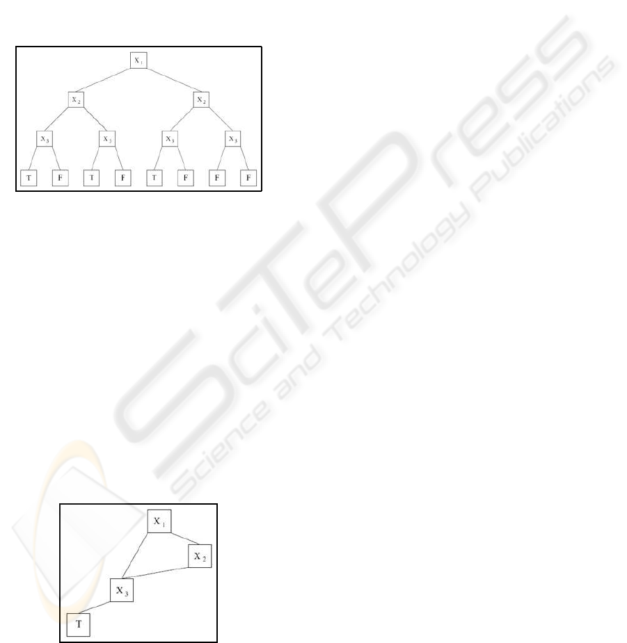
Figure 1: Representation of the boolean function
f(x
1
, x
2
, x
3
) = ¯x
1
· ¯x
2
· ¯x
3
+ ¯x
1
· x
2
· ¯x
3
+ x
1
· ¯x
2
· ¯x
3
.
As an example, Figure 1 shows the OBDD for the
boolean function f(x
1
, x
2
, x
3
) = ¯x
1
· ¯x
2
· ¯x
3
+ ¯x
1
· x
2
·
¯x
3
+ x
1
· ¯x
2
· ¯x
3
.
Usually, OBDDs are also reduced (ROBBD) by
merging isomorphic subgraphs and eliminating nodes
having two isomorphic children. In this way, any
boolean formula f can be represented by an unique
and very compact rooted, acyclic and directed graph.
The size of a reduced BDD is determined both by
the function being represented and by the chosen or-
dering of the variables. Thus, a correct variable order-
ing is of crucial importance to gain the best “reduction
factor”. The problem of finding the best variable or-
dering is NP-hard, but there exist efficient heuristics
to tackle the problem.
Figure 2: The OBDD in Figure 1 after removal of duplicate
nodes and redundant tests.
Figure 2 shows the reduced version of the OBDD
in Figure 1. Note that all the paths leading to F have
been actually removed from the graph, since they are
simply the complement of those leading to T.
A useful way to see BDDs, that will be used in
this paper, is that they encode the compressed repre-
sentation of a relation. However, unlike other com-
pression techniques, the actual operations on BDDs
are performed directly on that compressed represen-
tation, i.e. without decompression. Details on this
issue are given in Section 3.
3 BOOLEAN ENCODING OF
NUMERICAL CONTROLLERS
OBDDs can be used to create some kind of com-
pressed representation of any data that can be en-
coded as a logical expression. In this Section, we
describe how a numerical controller can be seen as
a boolean formula, and give details on the actual
OBDD-based compression algorithm that has been
implemented. Moreover, we give some informa-
tion on how the OBDD-compressed controller can
be efficiently queried and transformed in a hardware-
embeddable form.
3.1 Boolean Encoding of the Controller
Table
As already said, an OBDD can be actually seen
as a compact representation of a relation. On the
other hand, a controller table containing a set of
(state,action) pairs represents a relation R = {(s, a)|a
is the action associated to s in the controller table} be-
tween states and actions. Since BDDs encode formu-
las, it may be useful to represent R through its charac-
teristic function C
R
defined as follows:
C
R
(s, a) =
T if (s, a) ∈ R
F otherwise
Now, to write a definition of C
R
as a boolean for-
mula, we first have to represent its arguments, i.e.,
states and actions, in terms of logic variables. To this
aim, we expand them to their binary memory repre-
sentation.
Let suppose that states are n-bit values and actions
are m-bit values. We write s[i] and a[i] to denote the
ith bit of state s and action a,respectively.
Let x
i
, i = 1. . . n and y
j
, j = 1. . . m be n + m
boolean variables. A state s is then be represented
by the formula
OBDD COMPRESSION OF NUMERICAL CONTROLLERS
45

f
s
(x
1
, . . . , x
n
) =
^
i=1...n
l
i
where l
i
=
x
i
if s[i] = 1
¯x
i
if s[i] = 0
Each f
s
is a boolean formula in n variables that is
true if and only if its variables are assigned with the
bits of s (denoting, as usual, the boolean true with 1
and the boolean false with 0). In the same way, an
action a corresponds to the formula
f
a
(y
1
, . . . , y
m
) =
^
i=1...m
l
i
where l
i
=
y
i
if a[i] = 1
¯y
i
if a[i] = 0
.
Therefore, the controller characteristic function
C
R
can be encoded by the boolean formula
f
R
(x
1
, . . . , x
n
, y
1
, . . . , y
m
) =
_
(s,a)∈R
( f
s
∧ f
a
)
f
R
is a boolean formula in n+ m variables that is
true if and only if the variable assignment corresponds
to the encoding of a (s,a) pair for which R(s, a) holds.
For example, assume that the controller table con-
tains the following2-bit states s = 00, s
′
= 01, s
′′
= 10,
with the following associated 1-bit actions u = 0, u
′
=
0, u
′′
= 1. Then the formula for the characteristic rela-
tion would be f
R
= ¯x
1
· ¯x
2
· ¯y
1
+ ¯x
1
· x
2
· ¯y
1
+ x
1
· ¯x
2
· y
1
.
3.2 Algorithm for the Logic Encoding of
Numerical Controllers
BDD BDD_encoding(controller_table CTRL) {
read number
N
of entries in CTRL;
read number
n
of bits in each state of CTRL;
read number
m
of bits in each action of CTRL;
foreach j = 1. .. n
create boolean variable
x
j
;
foreach j = 1. .. m
create boolean variable
y
j
;
BDD
f
R
;
foreach i = 1.. . N
{
BDD E,
f
s
,
f
a
;
foreach j = 1. .. n //encode state bits
if
(bit(CTRL[i].state,j) == 1)
f
s
=
f
s
∧ x
j
;
else f
s
=
f
s
∧ ¯x
j
;
foreach j = 1. .. m //encode action bits
if
(bit(CTRL[i].action,j) == 1)
f
a
=
f
a
∧ y
j
;
else f
a
=
f
a
∧ ¯y
j
;
E =
f
s
∧ f
a
;
f
R
=
f
R
∨
E;
//disjunction of entries
}
return f
R
;}
Figure 3: Algorithm for the logic encoding of numerical
controllers.
The encoding algorithm, whose pseudocode is
shown in Figure 3, implements the technique de-
scribed in the previous Section.
After reading the number of bits in the controller
states and actions, the
BDD encoding
procedure cre-
ates the corresponding set of boolean variables x
i
and
y
i
, respectively.
Then, for each entry of the controller table, a new
BDD E is created as the appropriate conjunction of
the state and action variables. In particular, the code
checks every bit in the state and adds to the BDD f
s
a conjunction with the corresponding variable, in its
positive or negated form, based on the value of the bit.
The process is then repeated for the action bits in the
BDD f
a
, and finally E is obtained as f
s
∧ f
a
.
The BDD E is then added to the final BDD f
R
using a disjunction. When all the controller entries
have been processed,
BDD encoding
returns f
R
.
As we can see, the algorithm is actually very sim-
ple, since all the BDD manipulation is done by the
external BDD package. In particular, our implemen-
tation uses the CUDD (CUDD Web Page, 2007) BDD
manipulation package. Such package provides a large
set of operations on BDDs and many variable dy-
namic reordering methods, which are crucial to gain
the highest possible compression factor (Section 2).
Note that, to ensure the correctness of our ap-
proach, we also developed a parallel-query algorithm
that tests for correctness and completeness the BDD-
encoded controller f
R
with respect to the original
numerical controller CTRL. This procedure simply
compares the results obtained by querying the un-
compressed and the compressed controller with all the
states in the controller table.
3.3 Querying the Encoded Controller
Once we have compressed the controller table in a
BDD f
R
, we must show how this information can be
accessed by the controller itself to perform its task.
There are several ways to do this.
A first method relies on the fact that the generated
BDD actually encodes a function from states to ac-
tions. In other words, given a state, there is only one
action associated to such state in the controller table.
At the BDD level, this means that if we restrict the
BDD by assigning to the variables x
1
. . . x
n
the bits of
a particular state s, then the resulting BDD has only
one satisfying assignment, i.e., the one assigning to
y
1
. . . y
m
the bits of the corresponding action a.
Thus the action associated to a state can be found
by applying two operations (restriction and then de-
duction of satisfying assignments) on the BDD of f
R
.
However, since controllers must work in the quickest
ICINCO 2008 - International Conference on Informatics in Control, Automation and Robotics
46

and simplest possible way, we may consider an alter-
native query method that requires less runtime over-
head.
From the BDD of f
R
, we extract m different BDDs
f
1
R
. . . f
m
R
, one for each bit of the action, in the follow-
ing way.
f
i
R
(x
1
, . .. , x
n
) =
∃(y
1
. . .y
i−1
, y
i+1
, . .. y
m
)
f
R
(x
1
, . .. , x
n
, y
1
. . .y
i−1
, 1, y
i+1
, . .. y
m
)
In particular, in each f
i
R
we existentially abstract
all the action bit variables y
j
, j = 1. . . m except for
y
i
, which is assigned to the constant 1. The resulting
formula f
i
R
has n free variables x
1
. . . x
n
, which corre-
spond to the state bits.
If we assign x
1
. . . x
n
to the binary representation
of a state s, then f
i
R
is true if and only if there ex-
ists an action associated to s whose ith bit is 1. Since
the action associated to s, if it exists, is unique, f
i
R
actually returns the ith bit of the action associated to
s (assuming, as usual, that the logical true and false
correspond to the values 1 and 0, respectively).
Having these functions at hand, we can rebuild the
binary representation of the action a associated to the
state s by simply applying each f
i
R
to the encoding
of s, without any further runtime BDD manipulation.
The execution overhead is minimal in this case, since
the “computation” of the BDD value for a particular
variable assignment requires only a visit of the asso-
ciated graph.
3.4 BDD into C Code Translation
Embedding and querying the BDD-compressed nu-
merical controller within a small hardware or soft-
ware device is also an issue that can be addressed in
various ways.
Obviously, we cannot require CUDD or another
BDD-manipulation package to be present in the con-
troller. However, a BDD (or the set of BDDs obtained
using the technique described in Section 3.3) can be
simply translated in a C code fragment composed by
nested if-then-else statements.
The translation process is very straightforward
and requires only a visit of the OBDD graph. Let n
be a node of the OBDD associated with the logic vari-
able V(n), and let T(n) and E(n) be the two children
of n for V(n) = true and V(n) = false, respectively.
Then, we can define the C-translation of n as follows:
CT(n) =
IF
(V(n))
THEN
CT(T(n))
ELSE
CT(E(n))
This translation is linear in terms of the required
space, and the resulting representation can be easily
embedded in a (small) hardware device resulting in
good time performances.
4 EXPERIMENTAL RESULTS
To setup our experiments, we first have to fix some
BDD encoding parameters, namely the variable or-
dering in the boolean formulas and the dynamic re-
ordering method used by the BDD package.
Indeed, the BDD structure and therefore the com-
pression ratio can be influenced by the original or-
dering of the variables in the boolean formulas pre-
sented to the BDD package. In particular, we recall
that the variables in our BDDs are the state bit vari-
ables, namely x
i
, i = 1. . . n, and the action bit vari-
ables, y
i
, i = 1. . . m. Thus, we may consider the vari-
able orderings arising from all the possible combina-
tions of the following conditions:
• the state bit variables and the action bit variables
can be ordered with different endianness, that is
from the most significant bit to the least or vice-
versa;
• the state bit variables can be placed before the ac-
tion bit variables, after them or interleaved.
Namely, we can write the function f
R
of Section
3 with any of the ten variable orderings O1. . . O10
shown in Table 1. Note that in O9 and O10 we assume
n > m.
Table 1: Possible initial variable orderings.
O1 x
1
···x
n
y
1
···y
m
O2 x
1
···x
n
y
m
···y
1
O3 x
n
···x
1
y
1
···y
m
O4 x
n
···x
1
y
m
···y
1
O5 y
1
···y
m
x
1
···x
n
O6 y
1
···y
m
x
n
···x
1
O7 y
m
···y
1
x
1
···x
n
O8 y
m
···y
1
x
n
···x
1
O9 x
1
y
1
x
2
y
2
···x
m
y
m
x
m+1
···x
n
O10 x
n
, y
m
x
n−1
y
m−1
···x
m−n
y
1
x
m−n−1
···x
1
Moreover, variables can be dynamically reordered
by the BDD package during the construction of the
final BDD. In our experiments, we used the fourteen
dynamic reordering methods R1. . . R14 offered by the
CUDD package and shown in Table 2.
In the following experiments we tried all the pos-
sible combinations between initial variable orderings
and dynamic reordering methods, choosing each time
the one that produces the better compression ratio.
All the experiments were performed on a 2.66GHz
Pentium 4 with 1GB RAM.
OBDD COMPRESSION OF NUMERICAL CONTROLLERS
47
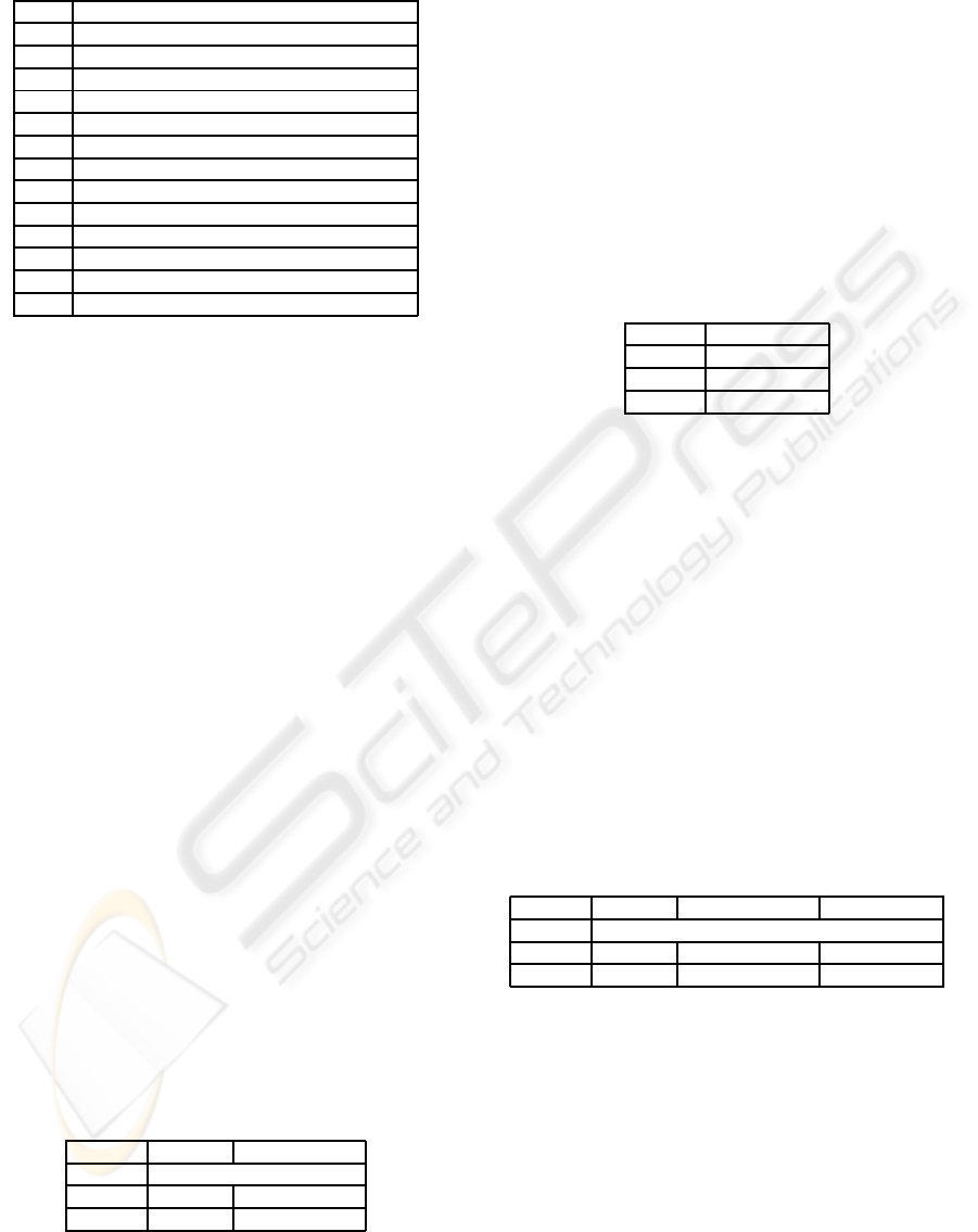
Table 2: CUDD variable reordering methods.
R1 Random reordering
R2 Random pivot reordering
R3 Sift
R4 Converging sifting
R5 Symmetric sifting
R6 Converging symmetric sifting
R7 Group sifting
R8 Converging group sifting
R9 Window permutation (size 2)
R10 Window permutation (size 3)
R11 Window permutation (size 4)
R12 Converging window permutation (size 2)
R13 Converging window permutation (size 3)
R14 Converging window permutation (size 4)
4.1 Inverted Pendulum Controller
The first case study is the numerical controller for
the inverted pendulum problem (Kreisselmeier and
Birkholzer, 1994), where the controller has to bring
the pendulum to equilibrium by applying a torque in
the shaft.
The optimal numerical controller was generated
using the dynamic programming method described
in (Kreisselmeier and Birkholzer, 1994). Table 3
shows the details of such controller. In the table, row
Entries indicates the number of controller entries (i.e.,
controlled states) and row Size-column Normal indi-
cates the controller table size in Kilobytes. Moreover,
to compare the effectiveness of the BDD compression
with respect to the common compression techniques,
we also show the size of the controller table com-
pressed by the LZ77-based (Ziv and Lempel, 1977)
algorithm of gzip (GZip Web Page, 2007) (row Size-
column LZ, where the relative size of the compressed
file is also shown as a percentage) and the average
controller access time in milliseconds for both the un-
compressed and the compressed representations (row
Time-column normal and row Time-column LZ, re-
spectively). Note that, as we expect, access times for
the LZ-compressed controller are very high since, in
the worst case, the controller must be completely de-
compressed to find the required table entry.
Table 3: Numerical controller for the inverted pendulum.
Normal LZ
Entries 311618
Size 3043 1295 (42.6%)
Time 8 ms 657 ms
When BDD compression is applied to the con-
troller, we obtain BDDs whose size (in number of
graph nodes) is shown in Table 4 for each combina-
tion of variable initial ordering (O1. . . O10) and dy-
namic reordering (R1. . . R14).
Here, the smallest BDD (indicated by the bold
number in Table 4) has 61584 nodes. The actual
size in Kilobytes and the average access time for the
BDD-compressed controller are shown in Table 5. As
we can see, BDD compression reduces the controller
26.5% more than LZ, and has also better access times
than the LZ-compressed version, since it does not re-
quire any decompression to read the table entries.
Table 5: BDD-compressed numerical controller for the in-
verted pendulum.
BDD
Entries 311618
Size 489 (16.1%)
Time 1 ms
4.2 Truck and Trailer Obstacles
Avoiding Controller
In the second case study, we consider the controller
for the truck and trailer obstacles avoiding problem.
Namely, the controller has to back a truck with a
trailer up to a specified parking place starting from
any initial position in the parking lot. Moreover, the
parking lot contains some obstacles, which have to
be avoided by the truck while maneuvering to reach
the parking place. Corrective maneuvers are not al-
lowed, that is the truck cannot move forward to back-
track from an erroneous move.
Table 6: Results for the truck and trailer obstacles avoiding
controller.
Normal LZ BDD
Entries 3256855
Size 71650 22644 (31.6%) 7038 (9.8%)
Time 89 ms 3173 ms 108 ms
The numerical controller was generated with the
CGMurϕ tool (CGMurphi Web Page, 2006; Della
Penna et al., 2007b). Results are in Table 6. As we
can see, the controller has a very big size. However,
the best BDD compression scheme (O5,R5) is able to
reduce the size of the controller up to a 90.2% space
savings, that is 21.8% more than using LZ77 com-
pression. Moreover, the BDD compression continues
to win also with respect to the access times.
ICINCO 2008 - International Conference on Informatics in Control, Automation and Robotics
48
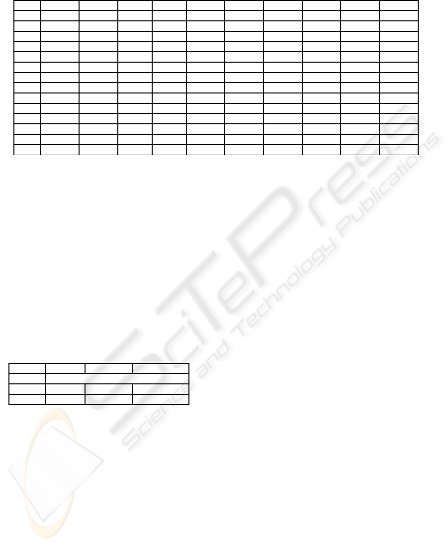
Table 4: Number of nodes in the BDD for the inverted pendulum controller with respect to different variable orderings.
O1 O2 O3 O4 O5 O6 O7 O8 O9 O10
R1 92490 108474 65382 64012 156872 83808 149943 86957 92013 145877
R2 142012 145654 66711 78029 130315 79575 144583 89528 148037 142432
R3 65842 61588 65842 61584 138377 75360 145181 143181 65854 127241
R4 65842 71314 70691 61584 130355 71313 75427 135580 65842 65843
R5 65842 65848 70774 70770 144310 70773 144422 70776 65865 142677
R6 65842 65860 70777 70770 135575 70773 135573 70773 65860 130348
R7 66759 66555 92830 61798 144268 61586 136870 61594 69198 65865
R8 65842 61594 75420 61584 145172 61586 135575 61586 65868 65863
R9 92295 92279 65441 61873 163149 121083 255309 121307 101164 178482
R10 76724 77231 61584 61588 134758 122539 143860 78044 79227 142072
R11 72724 72781 61584 61584 134023 122157 134254 106597 77295 134723
R12 81329 98992 61630 61641 134162 128731 138481 79723 86284 136761
R13 77034 65868 61584 61584 134023 123547 134275 111460 66122 134257
R14 65842 65868 61584 61584 134275 77960 134275 116568 68455 134079
4.3 Inverted Pendulum on a Cart
Controller
The last case study is the numerical controller for
the inverted pendulum on a cart problem (Junge and
Osinga, 2004). The system consists of a planar in-
verted pendulum on a cart that moves under an ap-
plied horizontal force, constituting the control. The
position of the pendulum is measured relative to the
position of the cart as the offset angle from the verti-
cal upright position. The controller goal is to set such
angle to zero.
Table 7: Results for the inverted pendulum on a cart con-
troller.
Normal LZ BDD
Entries 151394
Size 1478 90 (6.1%) 215 (14.6%)
Time 3 ms 206 ms 1 ms
The numerical controller was generated with the
CGMurϕ tool. Results are in Table 7. The number
of controller entries is very small with respect to the
previous two case studies. We see that on a small con-
troller the BDD compression has a lower compression
ratio than LZ, but always better access times (1ms vs.
206ms), since it does not require any decompression
to read the table entries.
5 CONCLUSIONS
In this paper, we presented an OBDD based compres-
sion algorithm for numerical controllers. The com-
pression algorithm is completely automatic and can
be applied to the (state,action) tables generated by any
numerical controller generation technique.
Our experiments show that this new algorithm has
a very high compression ratio (up to 10:1), that is of-
ten more than the ratio obtained on the same data by
the most common lossless compression techniques,
such as LZ77. Indeed, OBDD compression is not ac-
tually lossless, but rather “relation-invariant”. That is,
the OBDD compression leaves intact the behavior of
the state-action relation stored in the table. However,
by working on the logic encoding of the relation, the
OBDD is capable of optimizing the representation of
the relation, so reducing its size.
Moreover, accessing the entries of an OBDD-
compressed numerical controller does not require any
data decompression (as it would happen, e.g., with
LZ77), so the controller performances are very good.
Also in this case, the optimized representation gener-
ated by the OBDD sometimes allows to achieve ac-
cess times that are even better that those of an hash
function used on the uncompressed table.
Therefore, the BDD compression is a technique
that can be actually exploited to reduce the size of
numerical controllers, generating a compact structure
that is easy to store and query. This would allow, e.g.,
to use high precision controllers even in limited de-
vices.
Indeed, we are currently studying and implement-
ing algorithms that create embeddable and executable
forms of the OBDD-compressed controllers. The
OBDD-to-C methodology sketched in section 3.4 is
only the first step, as we intend to design a transla-
tion process to directly create an optimized VHDL
(Pedroni, 2004) circuit description from the OBDD.
In this way, we would have a completely automatic
methodology to generate, from any numerical con-
troller, a small executable definition ready to be em-
OBDD COMPRESSION OF NUMERICAL CONTROLLERS
49

bedded in the hardware.
Finally, a last point we want to investigate is the
relationship between the compression obtained with
the use of the OBDDs and the reduction of fuzzy con-
trol systems by means of a hierarchical approach (see
e.g. (Stufflebeam and Prasad, 1999)). Indeed, there is
an evident correspondence between, on one hand, the
search of the best ordering of variables needed for the
OBDD compression and, on the other, the hierarchi-
cal decompositioninto subsystems of a fuzzy system.
REFERENCES
Bryant, R. (1986). Graph-based algorithms for boolean
function manipulation. IEEE Trans. on Computers,
C-35(8):677–691.
Burch, J. R., Clarke, E. M., McMillan, K. L., Dill, D. L.,
and Hwang, L. J. (1992). Symbolic model checking:
10
20
states and beyond. Inf. Comput., 98(2):142–170.
CGMurphi Web Page (2006).
http://www.di.univaq.it/magazzeni/cgmurphi.php.
Clarke, E. M., Grumberg, O., and Peled, D. A. (1999).
Model Checking. The MIT Press.
Cormen, T., Leiserson, C., Rivest, R., and Stein, C. (2001).
Introduction to Algorithms. MIT Press.
Cover, T. M. and Thomas, J. A. (2006). Elements of Infor-
mation Theory. Wiley.
CUDD Web Page (2007). http://vlsi.colorado.edu/ fabio/.
Della Penna, G., Fallucchi, F., Intrigila, B., and Magazzeni,
D. (2007a). A genetic approach to the automatic gen-
eration of fuzzy control systems from numerical con-
trollers. In AI*IA, volume 4733 of LNAI, pages 230–
241. Springer-Verlag.
Della Penna, G., Intrigila, B., Magazzeni, D., Melatti,
I., Tofani, A., and Tronci, E. (2006). Au-
tomatic generation of optimal controllers through
model checking techniques. In Proceedings of 3rd
International Conference on Informatics in Con-
trol, Automation and Robotics (ICINCO2006), to
be published in Informatics in Control, Automa-
tion and Robotics III, draft available at the url
http://www.di.univaq.it/magazzeni/cgmurphi.php.
Della Penna, G., Magazzeni, D., Tofani, A., Intrigila, B.,
Melatti, I., and Tronci, E. (2007b). Automatic syn-
thesis of robust numerical controllers. In ICAS ’07,
page 4. IEEE Computer Society.
Gr¨une, L. and Junge, O. (2005). A set oriented approach to
optimal feedback stabilization. Systems Control Lett.,
54(2):169–180.
GZip Web Page (2007). http://www.gzip.org/.
Hand, D. J., Mannila, H., and Smyth, P. (2001). Principles
of Data Mining. MIT Press.
Junge, O. and Osinga, H. (2004). A set oriented approach to
global optimal control. ESAIM Control Optim. Calc.
Var., 10(2):259–270 (electronic), 2004.
Kosko, B. (1992). Neural Networks and Fuzzy Systems.
Prentice Hall.
Kreisselmeier, G. and Birkholzer, T. (1994). Numerical
nonlinear regulator design. IEEE Transactions on Au-
tomatic Control, 39(1):33–46.
Leu, M. C. and Kim, T.-Q. (1998). Cell mapping based
fuzzy control of car parking. In ICRA, pages 2494–
2499.
Nelson, M. and Gailly, J. (1995). The Data Compression
Book. MT Books.
Pedroni, V. (2004). Circuit Design with VHDL. MIT Press.
Sekine, S., Imasaki, N., and Tsunekazu, E. (1995). Appli-
cation of fuzzy neural network control to automatic
train operation and tuning of its control rules. In Proc.
IEEE Int. Conf. on Fuzzy Systems 1993, pages 1741–
1746, Yokohama.
Stufflebeam, J. and Prasad, N. (1999). Hierarchical fuzzy
control. In Proceedings of IEEE International Fuzzy
Systems Conference, pages 498–503.
Ziv, J. and Lempel, A. (1977). A universal algorithm for
sequential data compression. IEEE Transactions on
Information Theory, 23(3):337–343.
ICINCO 2008 - International Conference on Informatics in Control, Automation and Robotics
50
