
NEAR OPTIMUM CONTROL OF A FULL CAR
ACTIVE SUSPENSION SYSTEM
Paolo Lino and Bruno Maione
Dipartimento di Elettrotecnica ed Elettronica, Politecnico di Bari, via Re David 200, 70125, Bari, Italy
Keywords:
Active suspension, Suspension control, Virtual prototyping, Near-optimum control, AMESim
c
.
Abstract:
In this paper, a near-optimum control strategy applied to a full car model equipped with an active suspension
system is presented. The control law is based on a reduced order model obtained by means of a modal
aggregation method, achieving a compromise between computational effort in deriving the control law and
system performances. To assess the controller performances, a virtual prototype of the suspension system is
developed by using AMESim, an advanced fluid-mechanic developing tool. The virtual prototype could be
assumed as a reliable model of the real system enabling to perform safer and cheaper tests than using the real
system. Simulation results show the effectiveness of the approach.
1 INTRODUCTION
A vehicle suspension system mainly aims to carry
the car and its weight, control the vehicle direction
of travel, keep the tires in contact with the road, and
reduce the effect of shock forces due to road distur-
bances, braking and entries into curves. Handling and
ride comfort can be significantly improved by using
active suspension systems instead of passive or semi-
active suspensions. More in details, passive suspen-
sion systems include spring and dampers character-
ized by static input-output relationships; semi-active
suspensions use dampers with a variable damping co-
efficient; active suspensions apply a force on car body
and wheels by means of an activeactuator. The design
process of control systems for active and semi-active
suspensions is usually carried on by considering quar-
ter car or half car models. The former only represents
the vertical motion of the car body, the latter includes
pitch or roll motions. Full car models give a more
detailed representation of the car dynamics by includ-
ing vertical displacement, pitch and roll dynamics at
the same time. Different approaches to active suspen-
sions control have been investigated by researchers,
which are mainly based on fuzzy logic, adaptive con-
trol, LQR control and H
∞
control, see (Yoshimura
et al., 1997; Yoshimura et al., 1999; Huang and Lin,
2003; Al-Holou et al., 2002; Fialho and Balas, 2002;
Alleyene and Hedrick, 1995; Hrovat, 1997) and the
references therein.
The main drawback in using lower order models is
that interactions between suspensions are neglected,
so that the control action cannot compensate angu-
lar accelerations or sensibly improve stability. On the
other hand, using simplified models makes the con-
troller design easier. In this paper, a compromise
between computational effort, detail in representing
the system behaviour and controller performances is
achieved by applying a near-optimum control strategy
to a full car model equipped with an active suspension
system. The controller performances are assessed by
a virtual prototype of the suspension system. The vir-
tual prototype could be assumed as a reliable model of
the real system enabling to perform safer and cheaper
tests than using the real system. Moreover, the inte-
gration of design and optimization processes of both
mechanical and control subsystems are made easier
by taking into account mutual interactions (Lino and
Maione, 2007), thus reducing the whole design effort.
The proposed design process consists in few steps.
Firstly, a 14
th
order full car analytical model is de-
veloped, representing vertical car body and wheels
motion, as well as pitch and roll angles dynamics.
Then, a reduced order model is derived by applying
a modal aggregation technique and used to develop
a near-optimum control strategy. Finally, the virtual
prototype of suspension system is built to validate the
controller performances.
The paper is organized as follows. Sections 2
and 3 describe the full car analytical model and the
virtual prototype of suspension system, respectively.
The near-optimum control strategy is then introduced
in Section 4. Some simulation results concerning the
controlled system are shown in Section 5. Finally,
46
Lino P. and Maione B. (2008).
NEAR OPTIMUM CONTROL OF A FULL CAR ACTIVE SUSPENSION SYSTEM.
In Proceedings of the Fifth International Conference on Informatics in Control, Automation and Robotics - SPSMC, pages 46-52
DOI: 10.5220/0001498200460052
Copyright
c
SciTePress
Section 6 gives some conclusions.
2 DYNAMICAL MODEL OF THE
FULL CAR SUSPENSION
SYSTEM
The full car model of a suspension system represents
the vehicle as a rigid body with seven degrees of free-
dom, which originate from translation motion along
axes, as well as rotational motions, i.e. pitch and
roll motions around center of gravity (COG) (Ikenaga
et al., 2000).
With reference to Fig. 1, by setting COG of the
car body as origin of axes, the vehicle body dynamics
can be described by the following equations:
m
c
¨z = f
fl
+ f
fr
+ f
rl
+ f
rr
I
pc
¨
θ = − f
fl
l
f
+ f
fr
l
f
+ f
rl
l
r
+ f
rr
l
r
I
rc
¨
φ =
1
2
f
fl
Tr−
1
2
f
fr
Tr+
1
2
f
rl
Tr+
1
2
f
rr
Tr
(1)
where z is the vertical displacement of car body COG,
f
fl
, f
fr
, f
rl
, f
rr
are the forces applied by front-left,
front-right, rear-left, rear-right suspensions on the car
body, respectively, θ and φ are the pitch and roll an-
gles, respectively, l
f
and l
r
are the distances from the
front and rear axles to car body COG, Tr is the wheels
track, m
c
is the car body mass, I
pc
and I
rc
are the pitch
and roll moments of inertia of the car body, respec-
tively.
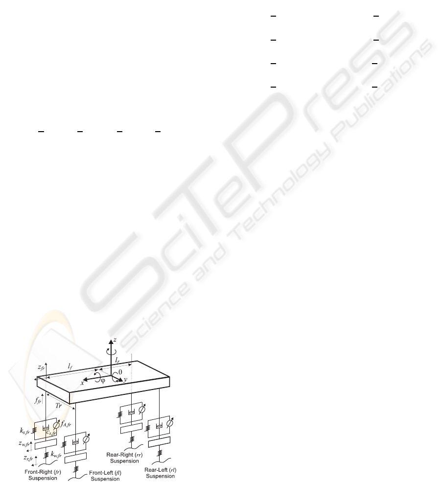
The force applied to the car body by each suspen-
sion can be computed as in the following:
f
i
= k
s,i
(z
w,i
− z
i
) + c
s,i
(˙z
w,i
− ˙z
i
) + f
A,i
m
w,i
¨z
w,i
= −k
s,i
(z
w,i
− z
i
) − c
s,i
(˙z
w,i
− ˙z
i
)+
− k
w,i
(z
w,i
− z
r,i
) − f
A,i
(2)
Figure 1: Vertical body model of the full car suspension
system.
where subscript i ∈ { fl, fr, rl,rr} characterizes the
four suspensions, z
w,i
and z
i
are the vertical displace-
ments of the wheel COG and car body corner, respec-
tively, m
w,i
is the wheel mass, k
s,i
and c
s,i
are the stiff-
ness and damping factor of the suspension, respec-
tively, k
w,i
is the wheel stiffness, and f
A,i
is the active
force applied by the controlled actuator.
The following equations express the vertical dis-
placement of car body corners in terms of z, θ and
φ:
z
fl
= z+
1
2
Tr· sinφ − l
f
sinθ ≈ z+
1
2
Tr· φ− l
f
θ
z
fr
= z−
1
2
Tr· sinφ − l
f
sinθ ≈ z−
1
2
Tr· φ− l
f
θ
z
rl
= z+
1
2
Tr· sinφ + l
r
sinθ ≈ z+
1
2
Tr· φ+ l
r
θ
z
rr
= z−
1
2
Tr· sinφ + l
r
sinθ ≈ z−
1
2
Tr· φ+ l
r
θ
(3)
where the approximations hold for small variations of
pitch and roll angles. Combining equations (1), (2)
and (3) results in a system of differential equations of
the form:
m
c
¨z
c
= f
1
(z
c
, ˙z
c
,z
w,i
, ˙z
w,i
,φ,
˙
φ,θ,
˙
θ, f
A,i
)
I
pc
¨
θ = f
2
(z
c
, ˙z
c
,z
w,i
, ˙z
w,i
,φ,
˙
φ,θ,
˙
θ, f
A,i
)
I
rc
¨
φ = f
3
(z
c
, ˙z
c
,z
w,i
, ˙z
w,i
,φ,
˙
φ,θ,
˙
θ, f
A,i
)
(4)
Equations (4), together with those of wheels vertical
displacements:
m
r
¨z
w,i
= f
4,i
(z
c
, ˙z
c
,z
w,i
, ˙z
w,i
,z
r,i
,θ,
˙
θ,φ,
˙
φ, f
A,i
) (5)
represent the full car dynamics under the action of
road disturbances and actuation forces. The design of
a control law can be simplified by putting equations
(4) and (5) in a state space form:
˙
x = Ax+ Bf+ Hd, (6)
where f = [ f
A, fl
, f
A, fr
, f
A,rl
, f
A,rr
]
T
is the vector of ac-
tuation forces, d = [z
r, fl
,z
r, fr
,z
r,rl
,z
r,rr
]
T
is the vector
of road disturbances, and x is the state vector, com-
posed of vertical displacements, pitch and roll angles
and its derivatives.
A more accurate model of the suspension system
includes the actuators dynamics. In this paper, the hy-
draulic actuator described in (Rajamani and Hedrick,
1995) is considered. It consists of a cylinder with a
moving piston pushed by the pressure difference on
its upper and lower surfaces (Fig. 2).
The pressure difference is regulated by an elec-
tronic valve driven by the control system. Under the
assumption of a negligible piston inertia with respect
to high hydraulic forces, the actuation force is given
by:
f
A,i
= −A
y,i
(˙z
c,i
− ˙z
w,i
) + u
i
, (7)
NEAR OPTIMUM CONTROL OF A FULL CAR ACTIVE SUSPENSION SYSTEM
47

Figure 2: Hydraulic actuator for active suspensions.
where u is a linear function of the control pressure set
by acting on the electronic valve, and A
y,i
is a con-
stant parameter depending on the system geometry
and working fluid characteristics. By suitably intro-
ducing an E matrix, the system state space model be-
comes:
˙
x = (A+ BE)x+ Bu+ Hd, (8)
where u is the vector of control inputs u
i
.
3 VIRTUAL PROTOTYPE OF THE
SUSPENSION SYSTEM
As virtual environment for design integration, we
use AMESim
c
(Advanced Modelling Environment
for Simulation): a simulation tool, which is oriented
to lumped parameter modelling of components from
different physical domains, interconnected by ports
enlightening the energy exchanges between element
and element and between an element and its environ-
ment. It also guarantees a flexible architecture, capa-
ble of including new components defined by the users
(IMAGINE S.A., 2004).
The AMESim virtual prototype (Fig. 3) used to
evaluate the controller performances has been devel-
oped by employing the AMESim-Simulink interface
in Co-simulation mode: each suspension-wheel sub-
system is modelled within the AMESim environment;
the car body dynamical equations (1) are solved using
MATLAB. AMESim and Simulink cooperate by inte-
grating the relevant portions of models.
The main components of each suspension-wheel
subsystem are the Mass block with stiction and
coulomb friction and end stops, which computes the
wheel dynamics through the Newtons second law of
motion, the Mechanical spring and dumper comput-
ing the elastic and damping forces of suspensions and
wheels depending on nonlinear stiffness and damping
coefficients, the Piston with moving body, represent-
ing the actuator hydraulic circuit dynamics and com-
puting the pressure forces acting upon the upper and
lower piston surfaces, and the 3 positions hydraulic
control valve modelling the electro-hydraulic circuit
driving the actuator.
The pressure dynamics inside cylinders are com-
puted as a function of intake and outtake flows Q
in
,
Q
out
, as well as of volume changes due to mechanical
part motions, according to the following equation:
dP
dt
=
K
f
v
ρ
dv
dt
− Q
in
+ Q
out
, (9)
where P and ρ are the working fluid pressure and den-
sity, respectively, and v is the taken up volume. Q
in
and Q
out
can be calculated by applying the energy
conservation law, which gives, for a generic Q:
Q = c
D
(ρ,η)Aρ
s
2|∆P|
ρ
sgn(∆P), (10)
where ∆P is the working fluid pressure difference
across the flow section A; sgn(∆P) is the sign func-
tion affecting the flow direction; the discharge coeffi-
cient c
D
accounts for nonuniform flow rates and flow
process non-isentropicity, depending on fluid density
ρ and cinematic viscosity η. Finally, the 3 positions
hydraulic control valve block models the controlled
valve as a second order spring-damp linear system.
To take into account the influence of inertia on
pitch and roll dynamics during brakes and entries into
a curve, the following equations are included in the
model:
I
PC
θ = m
c
h
cg
¨x
I
PC
φ = m
c
h
cg
¨y
, (11)
where h
cg
is the distance from the contact point be-
tween wheel and suspension to car body COG, and ¨x
and ¨y are the COG accelerations along x and y axes,
respectively.
4 THE NEAR-OPTIMUM
CONTROL STRATEGY
Given a system described by the state space equa-
tions:
˙x(t) = Ax(t) + Bu(t), x(0) = x
0
,
y(t) = Dx(t)
(12)
and a quadratic cost function:
J =
Z
∞
0
x(t)
T
Qx(t) + u(t)
T
Ru(t)
dt, (13)
being Q and R two positive semi-definite matrices,
it is well known that the Linear-Quadratic-Regulator
(LQR) problem consists in finding an input vector
u
∗
(t) = −Kx(t) minimizing the cost function J via
state-feedback (Dorato et al., 2000). The state feed-
back matrix K can be computed as:
K = R
−1
B
T
P, (14)
ICINCO 2008 - International Conference on Informatics in Control, Automation and Robotics
48
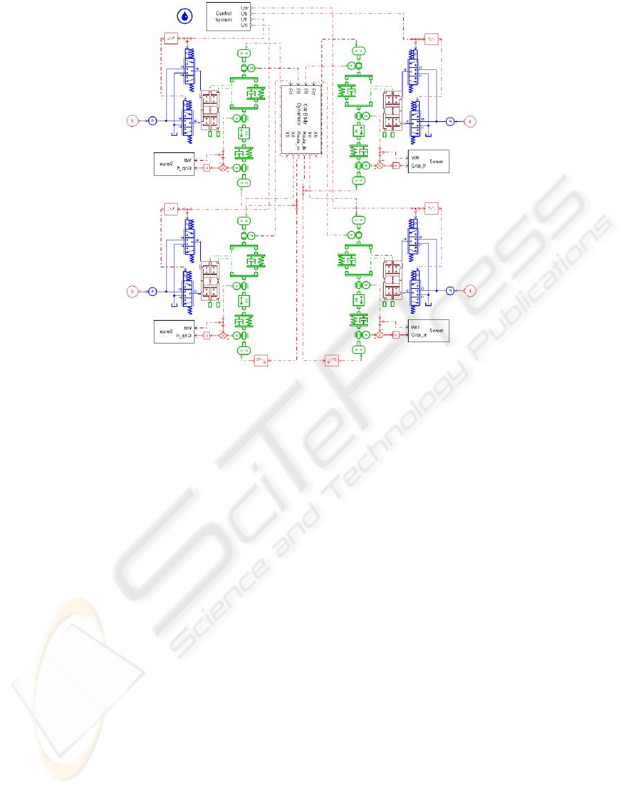
Figure 3: AMESim virtual prototype of the full car suspension system.
where P is the solution of the following matrix Riccati
equation:
A
T
P+ PA− PBR
−1
B
T
P+ Q = 0. (15)
Q and R matrices can be considered as weights on
state and control input, respectively, and affect the
value assumed by elements of matrix K. The Riccati
equation complexity directly depends on the system
order and its solution requests n(n + 1)/2 operations.
For a high order system it calls for a large compu-
tational effort, which could not be sustainable for on
line calculations; a solution consists in adopting large
scale system techniques to reduce problem complex-
ity and make the application of optimal control theory
easier (Jamshidi, 1983). These approaches, which are
based on reduction of order, perturbation of parame-
ters, decomposition of structure, hierarchical interac-
tion or decentralization of control, lead to near opti-
mality of system performance.
In this paper, the aggregation method based on the
modal approach is applied to reduce the model or-
der (Jamshidi, 1983). More in details, it neglects the
effect of non dominant modes to obtain a system of
aggregated states
ζ:
˙
ζ(t) = Fζ(t) + Gu(t),ζ(0) = ζ
0
˙
y(t) = Lζ(t)
(16)
by using a transformation matrix C:
ζ(t) = Cx(t), ζ(0) = Cx(0). (17)
The reduced order model matches the full order
model dynamics if the dynamic exactness condition
holds:
FC = CA
G = CB
LC = D.
(18)
By defining an error vector e(t) = ζ(t)−Cx(t), its dy-
namics is described by the equation
˙
e = Fe+ (FC−
CA)x+ (G− CB)u, which reduces to
˙
e = Fe if con-
ditions (18) hold. Provided that F is a positive definite
matrix, error reduces to 0 even for e(0) 6= 0.
To derive the aggregation matrix C, the modal ap-
proach exploits the system modal matrix M, whose el-
ements are the eigenvectors of state matrix A. Hence,
if arranging columns of matrix M by starting from
eigenvectors related to slowest dynamics, the reduced
order system matrices can be obtained using the fol-
lowing relationships:
F = M
l
SΛS
T
M
−1
l
C = M
l
SM
−1
G = CB
L ≈ DC
+
(19)
where M
l
is the nonsingular leading principal minor
of matrix M of order l, S = [I
l
0], being I
l
the Iden-
tity matrix, Λ is the Jordan matrix of A, and C
+
is the
pseudo-inverse of C.
NEAR OPTIMUM CONTROL OF A FULL CAR ACTIVE SUSPENSION SYSTEM
49

Considering the reduced order system, the Riccati
equation becomes:
F
T
P
a
+ P
F
− P
a
GR
−1
G
T
P
a
+ Q
a
= 0, (20)
so that the following control action is obtained:
u
a
(t) = −R
−1
G
T
P
a
ζ(t) = −R
−1
G
T
P
a
Cx(t)
= −K
a
x(t)
(21)
By pre- and post- multiplying eq. (20) by C
T
and C,
respectively, and considering the aggregation condi-
tions, it is straightforward to obtain:
A
T
(C
T
P
a
C) + (C
T
P
a
C)A+
− (C
T
P
a
C)BR
−1
B
T
(C
T
P
a
C) + C
T
Q
a
C = 0.
(22)
Equations (15) and (22) coincide provided that the
following positions hold:
P = C
T
P
a
C,
Q = C
T
Q
a
C.
(23)
Hence, the Q
a
matrix can be obtained as:
Q
a
= (CC
T
)
−1
CQC
T
(CC
T
)
−1
. (24)
Finally, K
a
matrix is obtained from F, G, Q
a
and R
matrices.
In this paper, a 6
th
order aggregated model is de-
rived from the full order suspension system and used
to derive the control law.
5 SIMULATION RESULTS
To evaluate the controller performances, a set of tests
is performed on the virtual prototype by applying
different road profiles. In particular, the following
benchmarks used in industrial practice are considered
(Canale et al., 2006):
•
Sine wave hole
profile: a sine profile hole with
0.03 m of amplitude and 6 m of width; for the
sake of brevity, only 30 and 90 Km/h car speeds
are considered in this paper;
•
Short back
profile: a positive step of road profile
with 0.02 m of amplitude and 0.5 m of width, with
a travelling speed of 30 Km/h;
•
Drain well
profile: a negative step variation of
road profile with 0.05 m of amplitude and 0.6 m
of width, with a traveling speed of 30 km/h.
Moreover, the system response in case of entry in
a curve or braking is analysed. The proposed con-
troller performances have been compared with those
obtained by using an active decoupled controller (Ike-
naga et al., 2000) and an LQR controller based on the
full order model. In particular, the control scheme
proposed in (Ikenaga et al., 2000) includes a ride con-
trol loop, for road disturbances rejection, and an atti-
tude control loop, for roll, pitch and vertical dynam-
ics regulation. To former includes an active filtering
feedback, the latter is based on a sky-hook control
strategy. A decoupling is performed to deal with the
under-actuation problem.
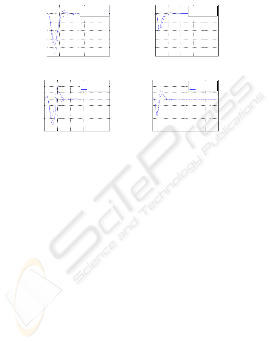
Figure 4 shows pitch and vertical displacement
dynamics when applying the sine wave hole road pro-
file. Since the road disturbance is symmetrically ap-
plied to left and right wheels, the roll dynamics is neg-
ligible and not displayed.
It is evident that the LQR controller guarantees
better performances than the near-optimum and the
decoupled controllers, in terms of overshoot and set-
tling time. Nevertheless, the near optimum controller
allows acceptable pitch angle and vertical displace-
ment dynamics, improving the results obtained with
the decoupled controller.
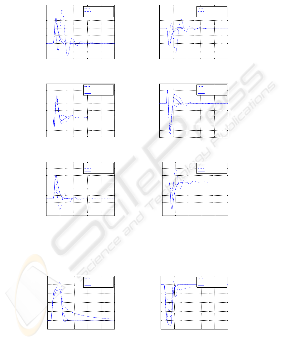
In Figure 5, the drain well and the short back
disturbances are only applied to left wheels, so that
the roll angle dynamics is excited. Simulation results
show that the LQR controller still guarantees a better
system behaviour for all conditions thanks to a prompt
control action, while the near-optimum controller im-
proves results obtained with the decoupled controller.
Finally, Figure 6 displays the effect of sudden
longitudinal and lateral accelerations determined by
braking (Fig. 6(a)), and entry into a curve (Fig. 6(b)),
which independently affect the pitch dynamics and
the roll dynamics, respectively.
In the former case, the near-optimum and the LQR
controllers show similar performances; in the latter
case, the near-optimum controller cannot reduce sig-
nificantly the roll angle overshoot. In general, the
decoupled controller cannot guarantee fast transients
due to actuator saturation; the near optimum and
LQR controller can suitably restrain the control ac-
tion thanks to a suitable choice of the performance in-
dex weights. To sum up, the near optimum controller
represents a compromise in terms of system perfor-
mances and complexity, while the LQR controller al-
ways shows the best performances.
6 CONCLUSIONS
In this paper, a near-optimum control strategy applied
to a full-car active suspension system has been pro-
posed. The design process relies on the use of a high
order analytical model, from which an aggregated low
order model is derived, and of a virtual prototype de-
veloped by using the AMESim simulation package.
ICINCO 2008 - International Conference on Informatics in Control, Automation and Robotics
50
0 1 2 3 4 5
−0.025
−0.02
−0.015
−0.01
−0.005
0
0.005
Sine Wave Hole 30 Km/h
Time [s]
Heave Position [m]
Decoupled C.
Optimal C.
Near−optimum C.
(a)
0 1 2 3 4 5
−0.025
−0.02
−0.015
−0.01
−0.005
0
0.005
Sine Wave Hole 90 Km/h
Time [s]
Heave Position [m]
Decoupled C.
Optimal C.
Near−optimum C.
(b)
0 1 2 3 4 5
−2.5
−2
−1.5
−1
−0.5
0
0.5
1
1.5
x 10
−3
Sine Wave Hole (30 Km/h)
Time [s]
Pitch Angle [rad]
Decoupled C.
Optimal C.
Near−optimum C.
(c)
0 1 2 3 4 5
−2.5
−2
−1.5
−1
−0.5
0
0.5
1
1.5
x 10
−3
Sine Wave Hole (90 Km/h)
Time [s]
Pitch Angle [rad]
Decoupled C.
Optimal C.
Near−optimum C.
(d)
Figure 4: Vertical displacement (a)-(b) and Pitch angle (c)-(d) dynamics for a sine wave hole road profile ran at 30 km/h and
90 km/h, respectively.
The virtual prototype represents a reliable benchmark
for evaluating the controller performances before the
implementation on the real system. Moreover, it can
be used for the integrated design of both mechanical
and control subsystems at the same time. As simula-
tion experiments have shown, the proposed controller
provides good performances, despite the low compu-
tational effort required.
REFERENCES
Al-Holou, N., Lahdhiri, T., Joo, D., Weaver, J., and
Al-Abbas, F. (2002). Sliding mode neural net-
work inference fuzzy logic control for active suspen-
sion systems. IEEE Transactions on Fuzzy Systems,
10(2):234–246.
Alleyene, A. and Hedrick, J. (1995). Nonlinear adaptive
control of active suspensions. IEEE Transactions on
Control Systems Technology, 3(1):94–101.
Canale, M., Milanese, M., and Novara, C. (2006).
Semi-Active Suspension Control Using ’Fast’ Model-
Predictive Techniques. IEEE Transactions on Control
Systems Technology, 14(6):1034–1046.
Dorato, P., Abdallah, C., and Cerone, V. (2000). Linear
Quadratic Control: An Introduction. Krieger Publish-
ing Company, Melbourne.
Fialho, I. and Balas, G. (2002). Road adaptive active sus-
pension design using linear parameter-varying gain-
scheduling. IEEE Transactions on Control Systems
Technology, 10(1):43–54.
Hrovat, D. (1997). Survey of Advanced Suspension Devel-
opments and Related Optimal Control Applications.
Automatica, 33(10):1781–1817.
Huang, S. and Lin, W. (2003). Adaptive fuzzy controller
with sliding surface for vehicle suspension control.
IEEE Transactions on Fuzzy Systems, 11(4):550–559.
Ikenaga, S., Lewis, F., Campos, J., and Davis, L. (2000).
Active suspension control of ground vehicle based on
a full-vehicle model. In ACC 2000, Proceedings of the
2000 American Control Conference.
Jamshidi, M. (1983). Large-Scale Systems: Modeling and
Control. Elsevier Science Ltd, Amsterdam.
Lino, P. and Maione, B. (2007). Integrated design of a
mechatronic system - the pressure control in common
rails. In ICINCO 2007, Proceedings of the Fourth In-
ternational Conference on Informatics in Control, Au-
tomation and Robotics, Angers, France.
Rajamani, R. and Hedrick, J. (1995). Adaptiver Observers
for Active Automotive Suspensions: Theory and Ex-
periment. IEEE Transactions on Control Systems
Technology, 3(1):86–93.
IMAGINE S.A. (2004). AMESim User Manual v4.2.
Roanne, France.
Yoshimura, T., Isari, Y., Li, Q., and Hino, J. (1997). Active
suspension of motor coaches using skyhook damper
and fuzzy logic control. Control Engineering Prac-
tice, 5(2):175–184.
Yoshimura, T., Nakaminami, K., Kurimoto, M., and Hino,
J. (1999). Active suspension of passenger cars using
linear and fuzzy-logic controls. Control Engineering
Practice, (7):41–47.
NEAR OPTIMUM CONTROL OF A FULL CAR ACTIVE SUSPENSION SYSTEM
51
0 1 2 3 4 5
−1
−0.5
0
0.5
1
1.5
2
2.5
x 10
−3
Short back
Time [s]
Heave Position [m]
Decoupled C.
Optimal C.
Near−optimum C.
(a)
0 1 2 3 4 5
−8
−6
−4
−2
0
2
4
6
x 10
−3
Drain well
Time [s]
Heave Position [m]
Decoupled C.
Optimal C.
Near−optimum C.
(b)
0 1 2 3 4 5
−2
−1
0
1
2
3
4
5
x 10
−4
Short back
Time [s]
Pitch Angle [rad]
Decoupled C.
Optimal C.
Near−optimum C.
(c)
0 1 2 3 4 5
−10
−8
−6
−4
−2
0
2
4
x 10
−4
Drain well
Time [s]
Pitch Angle [rad]
Decoupled C.
Optimal C.
Near−optimum C.
(d)
0 1 2 3 4 5
−5
−3
−1
1
3
5
7
9
11
x 10
−3
Short back
Time [s]
Roll Angle [rad]
Decoupled C.
Optimal C.
Near−optimum C.
(e)
0 1 2 3 4 5
−0.025
−0.02
−0.015
−0.01
−0.005
0
0.005
0.01
0.015
Drain well
Time [s]
Roll Angle [rad]
Decoupled C.
Optimal C.
Near−optimum C.
(f)
Figure 5: Vertical displacement, pitch angle and roll angle dynamics when applying short back and drain well road distur-
bances; (a)-(c)-(e) short back disturbance applied ; (b)-(d)-(f) drain well disturbance applied.
0 2 4 6 8 10
−0.02
0
0.02
0.04
0.06
0.08
0.1
Braking
Time [s]
Pitch Angle [rad]
Decoupled C.
Optimal C.
Near−optimum C.
(a)
0 2 4 6 8 10
−0.1
−0.08
−0.06
−0.04
−0.02
0
0.02
Entrance into curve
Time [s]
Roll Angle [rad]
Decoupled C.
Optimal C.
Near−optimum C.
(b)
Figure 6: Pitch angle (a) and roll angle (b) dynamics in case of braking and entry into a curve, respectively.
ICINCO 2008 - International Conference on Informatics in Control, Automation and Robotics
52
