
DCT DOMAIN VIDEO WATERMARKING
Attack Estimation and Capacity Evaluation
O. Dumitru, M. Mitrea and F. Prêteux
Institut TELECOM / TELECOM & Management SudParis, ARTEMIS Departement, France
Keywords: DCT video watermarking, capacity, attack, pdf estimation, Gaussian mixtures.
Abstract: The first difficulty when trying to evaluate with accuracy the video watermarking capacity is the lack of a
reliable statistical model for the malicious attacks. The present paper brings into evidence that the attack
effects in the DCT domain are stationary and computes the corresponding pdfs. In this respect, an in-depth
statistical approach is deployed by combining Gaussian mixture estimation with the probability confidence
limits. Further on, these pdfs are involved in capacity computation. The experimental results are obtained on
a corpus of 10 video sequences (about 25 minutes each), with heterogeneous content.
1 INTRODUCTION
For property right identification purposes, the
watermarking techniques insert a mark into some
original media (e.g. a video). If the mark insertion
does not result in visual artefacts, the method
features transparency. If a pirate cannot eliminate
the mark without damaging the marked video, the
method features robustness (Cox & others, 2002).
In practice, the better the robustness, the worse
the transparency. In order to reach a balance
between these two constraints, the mark is inserted
into some spectral representations of the original
data, e.g. in the DCT (Discrete Cosine Transform).
A crucial issue is to compute the watermarking
capacity, i.e. the largest amount of information
which can be inserted into a video, for prescribed
transparency and robustness. The watermarking
capacity is computed as the capacity of the noisy
channel modelling the watermarking method,
Figure 1. According to this model, the mark is
sampled from the information source. The detection
is impaired by the noise sources: the original video
itself and the attacks. The side information
watermarking exploits the fact that the original video
is known at the insertion but unknown at the
detection. As such a noise source should not
decrease the channel capacity (Costa, 1983), the
attacks remain the restricting factor and their
intimate knowledge would grant accuracy in
capacity evaluation. The present paper focuses on
some real life attacks and models their effects in the
DCT domain. Note that attack modelling is not a
trivial task. Actually, any mathematical approach
should properly answer at least the following
questions:
1. Does a general statistical model for the
considered attack effects, independent with
respect to the video sequence, really exist?
2. When considering an individual video sequence,
does a reliable model exist for any (intra)frame
content and any (inter)frame dependency?
Positive answers at these first questions mean a
proof of stationarity concerning the attacks.
3. In case such a model exists, which is its pdf
(probability density function)? Although the
Gaussian law is generally considered, previous
studies rejected this popular assumption.
Figure 1: The watermarking model.
The paper has the following structure. After
having defined a set of random variables
corresponding to the attack effects, Section 2
presents the statistical investigation procedure.
Section 3 describes the experimental results. The
capacity evaluation is dealt with in Section 4 while
Section 5 concludes the paper. The Appendix
summarises some theoretical bases.
Channel
mar
k
original video
attack
mark
detection
239
Dumitru O., Mitrea M. and Prêteux F. (2008).
DCT DOMAIN VIDEO WATERMARKING - Attack Estimation and Capacity Evaluation.
In Proceedings of the Fifth International Conference on Informatics in Control, Automation and Robotics - RA, pages 239-244
DOI: 10.5220/0001498302390244
Copyright
c
SciTePress

2 INVESTIGATION PROCEDURE
2.1 Attack Effect Representation
Be there an L frame colour video. Each frame is
represented in the HSV space. The following steps
are applied to each frame (Mitrea & others, 2006):
Compute the DCT on the original V component.
Decreasingly sort the coefficients and record the
largest
R
values in a vector
o
n ; record their
corresponding locations in a vector
l .
Apply the DCT to the attacked
V component and
record the coefficients at the l locations into the
new vector, denoted by
a
n .
Compute the vector:
oa
nndifference −= .
A set of
L vectors of the same type as difference
(each of them with
R components) is thus obtained.
Be noise a vector with L components,
containing the values corresponding to an arbitrarily
chosen rank
r in the set of difference vectors:
],...,,[
21 L
nnnnoise = . Such a vector is sampled
from a random variable modelling the attack effects
in the
th
r
rank of the DCT hierarchy. To model the
attacks means to obtain the
pdf for the corresponding
random variable (a model for each rank).
2.2 Pdf Estimation for Attacks
There are many pdf estimation tools based on iid
(independent and identically distributed) data, but
thiey do not apply here. The
noise vector is
computed on successive (dependent) frames and the
a priori lack of support for attack stationarity can
raise suspicions about the data identical distribution.
Hence, a general estimation procedure should be
considered (Mitrea & others, 2007):
Eliminate the data dependency. Sample the
],...,,[
21 L
nnnnoise = vector with a D period.
Shift the sampling origin and get
D iid data sets
],...,,[],...,,[
)1(
21
iDNiDi
N
iii
nnnxxx
+−+
= ,
where
Di ,...,2,1=
and
DLN /= .
Extract partial information from each iid data
set.
Obtain )(
ˆ
xp
i
( Di ,...,2,1
=
) by Gaussian
mixture estimation (Appendix).
Extract global information. Apply the Gaussian
mixture estimation to the
noise vector and obtain
)(
ˆ
xp
av
(an average model).
Define the model. First, define a similarity
measure between two
pdfs, eq. (1):
∑
∫
∑
∫
=
=
⎟
⎠
⎞
⎜
⎝
⎛
⎟
⎠
⎞
⎜
⎝
⎛
−
=
S
s
I
S
s
I
s
s
dxxv
dxxvxu
xvxum
1
2
1
2
)(
))()((
))(),((
,
(1)
where
s
I , Ss ,...2,1
=
is a subdivision of the
];[
maxmin
xx interval on which the u and
v
pdfs take non-zero values. Secondly, define the
attack model as
(.)
ˆ
p which is the iid estimate
closest to the
(.)
ˆ
av
p in the (.)m sense:
))(
ˆ
),(
ˆ
(minarg)(
ˆ
xpxpmxp
i
av
i
= .
(2)
Evaluate the model accuracy. Calculate the
average similarity measure between each of the
D pdfs and the (.)
ˆ
p model, eq. (3):
∑
=
=
D
i
i
xpxpm
D
Error
1
))(
ˆ
),(
ˆ
(
1
.
(3)
If this procedure is successful when applied to an
individual video (Section 3.1), then positive answers
to the last two questions in the Introduction are
obtained. A positive answer to the first question is
obtained iff. the same model is obtained for different
video sequences (Section 3.2).
3 EXPERIMENTAL RESULTS
The corpus contains 10 video sequences (64 Kbit/s),
each of them of
35000
=
L frames (about 25
minutes each). The content is heterogeneous,
combining film, news, and home video excerpts.
The frame size is
80192 × pixels. The V
component is normalised to the
]1,0[
interval. The
DCT is individually applied to whole frames, and
the largest
360
=
R coefficients are investigated.
3.1 Model Computation
The model is computed for an arbitrarily chosen
video sequence. The following parameters are
considered:
250
=
D frames (i.e. 10s); 10=K pdfs
in the mixture;
200
=
iter
N iterations in the EM
algorithm;
20
=
S evenly distributed intervals.
Table 1 presents the models for three ranks (1,
150, 300) and three attacks (Gaussian filtering,
sharpening, and StirMark). In each case, the
)(
ˆ
xp
model is computed according to (2), its the
parameters (
kk
kP
σ
μ
,),( ) according to (A3) and
ICINCO 2008 - International Conference on Informatics in Control, Automation and Robotics
240
the corresponding errors to (3). Notice that each and
every time, the
Error values are lower than 0.04.
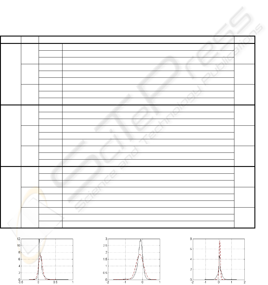
In order to illustrate the results in Table 1,
Figure 2 depicts in continuous line the models for
one rank (
300=r ) and the three attacks. For
comparison, Figure 2 also represents (in dashed line)
the Gaussian
pdf with the same mean values and
variances as the computed models.
The same results were obtained for each of the
10 video sequences in the corpus and for each
investigated attack: the parameters were slightly
different but the errors were lower than 0.05.
The models, for all 360 ranks and for other
attacks (Frequency Model Laplacian Removal,
median filtering, small rotations, JPEG compression)
can be obtained by contacting the authors.
3.2 Model Validation
Up to now, the experimental results point to the
existence of a model for the attack effects on a
particular video sequence and estimate this model
(
i.e. elucidates the second & third questions in the
Introduction).
Table 1: Statistical model for the watermarking attacks in the DCT hierarchy.
Attack
Rank
Model parameters Error
P(k) 0.076 0.072 0.228 0.095 0.021 0.096 0.071 0.133 0.120 0.083
μ(k) 0.274 0.319 0.214 0.305 0.788 0.283 0.330 0.052 0.440 0.374
r = 1
σ(k) 0.110 0.118 0.031 0.116 0.037 0.112 0.108 0.055 0.091 0.112
0.035
P(k) 0.019 0.025 0.190 0.213 0.091 0.075 0.271 0.025 0.031 0.056
μ(k) 0.224 0.195 0.031 0.009 0.072 0.121 0.063 0.101 0.201 0.131
r=150
σ(k) 0.130 0.135 0.011 0.021 0.083 0.010 0.010 0.110 0.134 0.046
0.013
P(k) 0.080 0.044 0.048 0.146 0.056 0.038 0.041 0.284 0.093 0.164
μ(k) 0.131 0.096 0.094 0.066 0.083 0.091 0.090 0.023 0.062 0.055
Gaussian filtering
r=300
σ(k) 0.053 0.112 0.111 0.025 0.069 0.110 0.110 0.012 0.026 0.029
0.013
P(k) 0.319 0.057 0.083 0.066 0.095 0.056 0.101 0.073 0.074 0.071
μ(k) -1.478 -1.185 -2.325 -2.151 -2.341 -0.971 -2.424 -0.536 -2.347 -2.141
r = 1
σ(k) 0.284 0.789 0.557 0.604 0.551 0.747 0.441 0.648 0.549 0.606
0.020
P(k) 0.102 0.029 0.091 0.033 0.171 0.033 0.140 0.081 0.155 0.159
μ(k) -0.324 0.213 -0.124 -1.104 -0.080 -0.716 -0.063 -0.279 -0.078 -0.035
r=150
σ(k) 0.137 0.028 0.102 0.316 0.103 0.168 0.103 0.150 0.104 0.098
0.021
P(k) 0.054 0.151 0.283 0.105 0.078 0.067 0.073 0.098 0.023 0.063
μ(k) -0.211 -0.105 -0.106 -0.114 -0.369 -0.030 -0.115 -0.120 -0.905 -0.203
Sharpening
r=300
σ(k) 0.180 0.096 0.095 0.156 0.133 0.133 0.156 0.158 0.155 0.178
0.021
P(k) 0.070 0.087 0.105 0.116 0.097 0.100 0.059 0.131 0.069 0.161
μ(k) -0.480 0.075 -0.354 -0.289 -0.115 -0.389 -0.401 -0.348 -0.619 -0.150
r = 1
σ(k) 0.368 0.397 0.271 0.263 0.436 0.270 0.404 0.269 0.357 0.215
0.037
P(k) 0.235 0.083 0.043 0.096 0.070 0.149 0.087 0.048 0.075 0.109
μ(k) 0.036 -0.084 0.206 0.103 0.422 0.006 0.017 -0.096 0.092 0.124
r=150
σ(k) 0.084 0.204 0.027 0.063 0.073 0.100 0.136 0.203 0.155 0.146
0.019
P(k) 0.085 0.075 0.046 0.078 0.137 0.036 0.010 0.046 0.300 0.093
μ(k) 0.004 0.191 0.197 -0.003 0.192 0.165 -0.005 0.212 0.047 0.015
StirMark
r=300
σ(k) 0.144 0.193 0.192 0.141 0.074 0.195 0.140 0.189 0.036 0.148
0.018
Gaussian filtering Sharpening StirMark
Figure 2: The attack models (continuous line) and the corresponding Gaussian laws (dashed line) for the rank r=300.
DCT DOMAIN VIDEO WATERMARKING - Attack Estimation and Capacity Evaluation
241

The model independence w.r.t. the video sequence
and the estimation procedure is now to be
investigated.
First, it should be précised whether the model
computed on a particular video sequence can be
representative for the whole corpus or not. In this
respect, the investigation algorithm is resumed on
the rest of 9 video sequences from the corpus and
the corresponding models are computed. The errors
between the reference model and these new models
are evaluated according to three criteria: the
similarity measure in eq. (1), the Kullback-Leibler
divergence and the Hellinger distance (Appendix).
For each criterion, and for three ranks, the minimal,
maximal, and average errors are reported in Table 2.
The numerical values obtained for the distance in
eq. (1) ascertain a quite good accuracy (and
generality) for the model provided in Table 1: the
average errors are acceptably low, with one
exception, namely the Gaussian filtering. The
Kullback-Leibler divergence and the Hellinger
distance lead to acceptably small values for all the
attacks. In order to compute these three measures,
the following instantiations were made in eqs. (1),
(A4) and (A5):
)(xv is the reference pdf while )(xu
is, successively, each of the other 9 individual
models computed on the corpus. The interval
I
is
]3,3[
mixmixmixmix
I
σ
μ
σ
μ
∗+∗−= , where
mix
μ
and
mix
σ
are the mixture mean and variance.
Secondly, the concordance between the
maximum likelihood estimation (which is the basis
for the EM Gaussian mixture algorithm) and the
popular confidence limit estimation is checked. Note
that the EM Gaussian mixture estimation results in a
continuous
pdf while the confidence limit estimation
provides values for the probability that a random
variable takes values in a given interval, but not the
pdf itself. Consequently, the interval where the
Gaussian mixture
model takes non-zero values is
evenly divided into 10 sub-intervals. On the one
hand, confidence limits for the probability that the
noise effects would take values in these sub-intervals
are derived. On the other hand, the integral of the
Gaussian mixture model on the same sub-intervals
are computed. The experiments bring into evidence
that each and every time (
i.e. for each type of
investigated attack and for each rank) the integral on
the EM Gaussian model belongs to the
corresponding confidence limits.
This sub-section shows that an individual model
(Table 1), computed on a particular video sequence,
is valuable for all the video sequences involved in
the experiments and, moreover, that it does not
depend on the estimation procedure. This means a
positive answer to the first question in Introduction.
4 CAPACITY COMPUTATION
As discussed in Introduction, any side-information
watermarking technique can be modelled by a noisy
channel, where the mark is a sample from the
information source and the noise is represented by
the attacks. In order to evaluate the capacity of such
a channel, the eqs. (A7) and (A8) are considered.
For the capacity limits in eq. (A7), the noise power
N is the variance of the noise vector, Section 2.2.
The signal power
P was derived from transparency
constraints, so as to ensure a mark 30dB lower than
the original (unmarked) coefficients.
Table 2: The errors (minimal, maximal, average) between the reference model and the 9 models obtained on different video
sequences, for three ranks:
r = 1, r=150, and r = 300.
r = 1 r = 150 r = 300
Type Attack
Min Max Average Min Max Average Min Max Average
Gaussian filtering 0.662 0.758 0.710 0.058 0.216 0.137 0.071 0.153 0.112
Sharpening 0.109 0.148 0.128 0.028 0.065 0.046 0.055 0.087 0.071
Error
StirMark 0.077 0.093 0.085 0.065 0.109 0.087 0.084 0.131 0.108
Gaussian filtering 0.131 0.204 0.167 0.011 0.016 0.014 0.029 0.030 0.029
Sharpening 0.035 0.712 0.374 0.066 0.110 0.088 0.081 0.098 0.089
D
KL
.
StirMark 0.106 0.110 0.108 0.015 0.018 0.016 0.024 0.026 0.025
Gaussian filtering 0.054 0.075 0.064 0.006 0.014 0.010 0.006 0.010 0.008
Sharpening 0.213 0.255 0.234 0.009 0.019 0.014 0.015 0.015 0.015
D
HL
.
StirMark 0.025 0.029 0.027 0.002 0.003 0.002 0.004 0.004 0.004
ICINCO 2008 - International Conference on Informatics in Control, Automation and Robotics
242

The
1
N
entropic power was also estimated on the
o
n original coefficient vector. The bandwidth W
was computed as half the frame rate.
When considering the capacity value in eq. (A8),
the model provided by the present study (
i.e. the pdf
in Table 1) is considered as the noise
pdf )(np
N
.
The
)(xp
X
function giving the capacity value is
searched for by means of a numerical strategy.
Actually, it is considered that
)(xp
X
itself can be
represented as a mixture of 5 Gaussian laws, thus
restricting the searching to a space with 15
dimensions (5 weights, 5 means values and 5
variances). These 15 dimensions are not
independent. First, the sum of weights should
equal 1. Secondly, the mean of the mark (
i.e. the
mixture mean) is set to 0 (a generally accepted
assumption in watermarking). Thirdly, the mixture
variance was set so as to ensure a good transparency
(
i.e. 30dB lower than the host video).
The capacity values computed with the general
formula and with Shannon limits are shown in
Table 3. A general agreement between the two types
of capacity estimation can e noticed, with some
exceptions (for
1=
r
of Gaussian filtering, StirMark).
At the same time, the capacity estimation starting
from the attack models is compulsory when a certain
degree of precision is required: that capacity
evaluation by limits can lead at relative errors of
about 100% and larger!
Table 3: Capacity value and limits (lower and upper ) for
rank
r = 1, r = 150 and r=300.
Rank
Attack
Capacity
Gaussian
filtering
Sharpening StirMark
value 3.567 1.332 2.307
r = 1
limits
(3.632 ;
3.651)
(1.268 ;
1.725)
(2.394 ;
2.415)
value 0.339 0.251 0.259
r =
150
limits
(0.037 ;
0.949)
(0.004 ;
0.569)
(0.005 ;
0.273)
value 0.055 0.006 0.009
r =
300
limits
(0.018 ;
0.935)
(0.002 ;
0.621)
(0.002 ;
0.273)
5 CONCLUSIONS
The present paper brings into evidence that some
real life watermarking attack effects are stationary in
the DCT hierarchy and accurately estimates the
corresponding probability density functions. Then,
these models are involved in capacity evaluation.
From the applicative point of view, beyond
watermarking itself (
i.e. reaching the capacity limit
in a practical application), these results are the
starting point for a large variety of applications in
the multimedia content processing, as smart
indexing or in-band content enrichment, for
instance.
Further work will be also devoted to considering
the Blahut approach for watermarking capacity
evaluation.
ACKNOWLEDGEMENTS
This work is partially supported by the HD3D-IIO
project of the Cap Digital competitiveness cluster.
REFERENCES
Archambeau, C., Lee, J., Verleysen, M., 2003.
Convergence Problems of the EM Algorithm for
Finite Gaussian Mixtures, Proc. 11th European
Symposium on Artificial Neural Networks
, Bruges,
Belgium, pp. 99-106.
Archambeau, C., Verleysen, M., 2003. Fully
Nonparametric Probability Density Function
Estimation with Finite Gaussian Mixture Models,
Proc. ICAPR, Calcutta, India, pp. 81-84.
Archambeau, C., Valle, M., Assenza, A., Verleysen, M.,
2006. Assessment of Probability Density Estimation
Methods: Parzen Window and Finite Gaussian
Mixtures,
Proc. IEEE International Symposium on
Circuits and Systems
, Kos, Greece.
Basseville, M., 1996. Information: entropies, divergences
et moyennes,
Internal report–INRIA, N°1020.
Costa, M., 1983. Writing on dirty paper,
IEEE
Transactions on Information Theory
, Vol. IT-29, pp.
439-441.
Cox, I., Miller, M., Bloom, J., 2002.
Digital
Watermarking
, Morgan Kaufmann Publishers.
Dempster, A.P., Laird, N.M., Rubin, D.B., 1977.
Maximum Likelihood from Incomplete Data via the
EM Algorithm,
Journal of the Royal Statistical
Society, Series B
, Vol. 39, No. 1, pp. 1-38.
Dumitru, O., Duta, S., Mitrea, M., Prêteux, F., 2007.
Gaussian Hypothesis for Video Watermarking
Attacks: Drawbacks and Limitations,
EUROCON
2007
, Warsaw, Poland, pp. 849-855.
Dumitru, O., Mitrea, M., Preteux, F., 2007. Accurate
Watermarking Capacity Evaluation, Proc. SPIE, Vol.
6763, pp. 676303:1-12.
Mitrea, M., Prêteux, F., Petrescu, M., 2006. Very Low
Bitrate Video: A Statistical Analysis in the DCT
Domain, LNCS, Vol. 3893, pp. 99-106.
DCT DOMAIN VIDEO WATERMARKING - Attack Estimation and Capacity Evaluation
243

Mitrea, M., Dumitru, O., Prêteux F, Vlad, A., 2007. Zero
Memory Information Sources Approximating to Video
Watermarking Attacks, LNCS, Vol. 4705, pp. 409-423.
Trailovic, L., Pao, L., 2002, Variance Estimation and
Ranking of Gaussian Mixture Distribution in Target
Tracking Applications,
Proc. of the 41st IEEE Conf.
on Decision and Control
, Las Vegas – Nevada, USA,
pp. 2195-2201.
APPENDIX
A1 Pdf Estimation Tools
Be there ],...,,[
21 N
xxx a set of N experimental
data complying with the
iid model. Suppose that
these data are sampled from a random variable
X
whose
pdf )(xp
is unknown and should be
estimated. A
)(
ˆ
xp Gaussian mixture is a linear
combination of Gaussian laws and can approximate
any continuous
)(xp pdf (Archambeau & other,
2003):
∑
=
=
K
k
k
xpkPxp
1
)()()(
ˆ
,
(A1)
where
)
2
)(
exp(
2
1
)(
2
2
2
k
k
k
k
x
xp
σ
μ
πσ
−
−=
.
The number of mixtures
K
is pre-established by
the experimenter and
kk
kP
σ
μ
,),( are 3K
parameters to be estimated by the EM (expectation
maximisation) algorithm (Dempster & other, 1977),
based on a maximum likelihood criterion:
the E step:
)(
ˆ
)()(
)(
)(
)(
)(
)(
n
i
i
n
i
k
n
i
xp
kPxp
xkp
= ,
(A2)
the M step:
∑
∑
=
=
+
=
N
n
n
i
N
n
nn
i
i
k
xkp
xxkp
1
)(
1
)(
)1(
)(
)(
μ
,
∑
∑
=
=
+
+
⎟
⎠
⎞
⎜
⎝
⎛
−
=
N
n
n
i
N
n
i
k
nn
i
i
k
xkp
xxkp
1
)(
1
2
)1(
)(
)1(2
)(
)(
)(
μ
σ
∑
=
+
⋅=
N
n
n
ii
xkp
N
kP
1
)()1(
)(
1
)( ,
(A3)
where the (
i ) upper index denotes the current
iteration; the total number of iterations is also
subject to the experimenters choice.
The relationship among the parameters of the
individual Gaussian laws and the mixture parameters
is given in (Trailovic, Pao, 2002).
Alongside with the similarity measure defined in
eq. (1), two popular methods for
pdf comparison are
involved in the experiments (Basseville, 1996):
Kullback-Leibler divergence:
dx
xv
xu
xuvuD
I
KL
∫
=
)(
)(
log)(),(
2
;
(A4)
Hellinger distance:
(
)
∫
−=
I
HL
dxxvxuvuD
2
)()(
2
1
),( .
(A5)
A2 Capacity Evaluation Basis
The capacity of a continuous channel, whose input
and output information sources are denoted by
X
and
Y
is given by the Shannon’s formula (A6):
∫∫
=
2
1
2
1
),(max
)(
x
x
y
y
XY
xp
dxdyyxfC
X
,
(A6)
)()(
),(
log),(),(
2
ypxp
yxp
yxpyxf
YX
XY
XYXY
=
,
where
)(xp
X
and )(yp
Y
stand for the input and
output
pdfs, while ),( yxp
XY
is the joint pdf of
X
and
Y
. The
21
, xx and
21
, yy are the limits of the
intervals on which the input and output
pdfs have
non-zero values. In the case of a non-Gaussian
noise, Shannon derives some upper and lower limits,
eq. (A7):
1
2
1
1
2
loglog
N
NP
WC
N
NP
W
+
≤≤
+
,
(A7)
where
W is the channel bandwidth,
P
is the signal
power,
N is the noise power, and
1
N is the noise
entropy power (
i.e. the power of a white-type noise
which has the same bandwidth and entropy as the
considered noise).
When assuming the noise is additive and
independent, eq. (A6) becomes:
dydxyxgC
x
x
nx
nx
XY
xp
X
∫∫
+
+
=
2
1
22
11
),(max
)(
,
(A8)
∫
−
−
−=
2
1
)()(
)(
log)()(),(
2
n
n
XN
N
NXXY
dnnypnp
xyp
xypxpyxg
,
where the noise limits are
111
xyn −= and
222
xyn
−
=
(Dumitru, & others, 2007).
ICINCO 2008 - International Conference on Informatics in Control, Automation and Robotics
244
