ENERGY MODEL BASED CONTROL FOR FORMING

PROCESSES

Patrick Girard

Industrial Materials Institute, National Research Council, 75 Boulevard de Mortagne, Boucherville, Canada

Vincent Thomson

Mechanical Engineering, McGill University, 817 Sherbrooke St.W. Montreal, Canada

Keywords: Model based control, forming energy, simulation, real time identification, intelligent agents, on-line

diagnostics.

Abstract: Thermoforming consists of shaping a plastic material by deforming it at an adequate deformation rate and

temperature. It often exhibits abrupt switches between stable and unstable material behaviour that have

neither been identified nor controlled up to now. PID control, although adequate for simple parts, has not

been able to control very well the forming of complex parts and parts made of newer materials. In this

paper, the state parameters that allow the development of predictive models for the forming process and the

construction of control systems are identified. A robust, model based control system capable of in-cycle

control is presented. It is based on a simulator continuously tuned and supported in real time by intelligent

agents that incorporate diagnostic capabilities.

1 INTRODUCTION

Forming processes are widely used in a number of

industries, including automotive, aerospace and

home appliances. Forming is an apparently simple

process in which a sometimes pre-shaped sheet of

plastic material is first heated to the correct forming

temperature in a first phase, and then deformed in a

second phase at the correct strain rate, generally by

pressing it against a mould to impart a specific

shape. The deformation of the sheet is insured by

using either a vacuum or pressure at a given

temperature and deformation rate, sometimes with

the assistance of a mechanical plug. After the part is

ejected from the mould some additional, post-

processing steps may be required, such as cooling at

a controlled rate, or annealing to relieve the built in

stresses that were induced by this transformation

process.

Effective control of forming needs to address the

following issues.

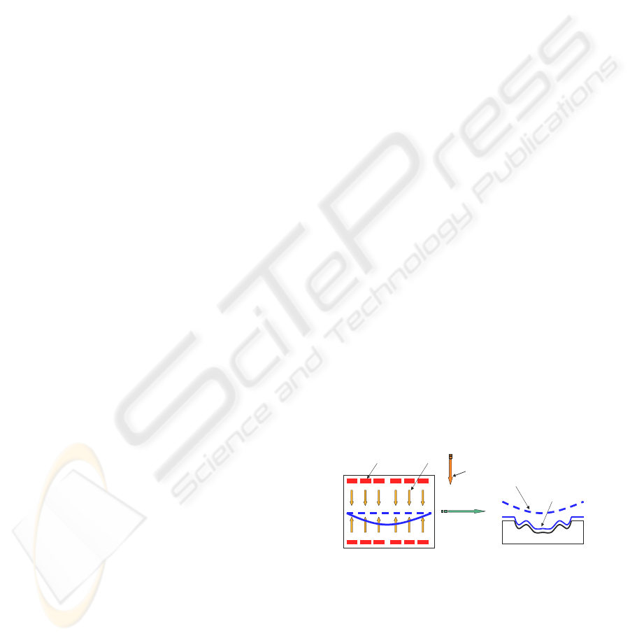
• How energy is transferred to the part can be

transformed into two separate processing

steps, first to bring it to the correct forming

temperature, and then to shape it (Figure 1).

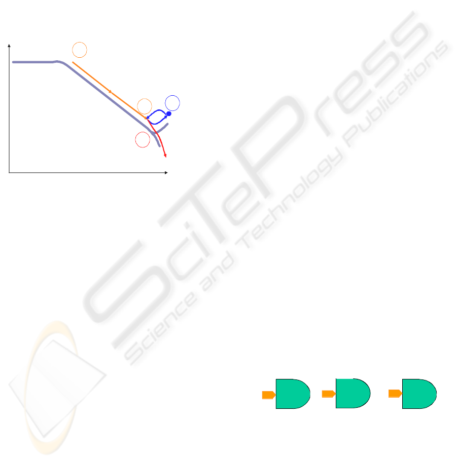
• Depending on the rate that the material

deforms, variations in the deformation rate

produce enormous changes in the viscosity of

the material, resulting in very high and

unstable variations of the energy required for

deformation as shown in Figure 2.

Heating elements

Radiation heatin

To Forming

Station

Initial Shape

Of Sheet

After Forming through

Pressure

Vacuum

Forming Station

2D Temperature scan

at exit of oven

Oven

Figure 1: The thermoforming process (Girard et al., 2005).

Up to now forming has been controlled in a very

empirical and indirect manner. For example, during

the heating phase of the sheet only the temperature

of the heating elements has been controlled. The rate

of deformation during forming is controlled by

applying pressure on the material either as a constant

Girard P. and Thomson V. (2008).

ENERGY MODEL BASED CONTROL FOR FORMING PROCESSES.

In Proceedings of the Fifth International Conference on Informatics in Control, Automation and Robotics - ICSO, pages 51-59

DOI: 10.5220/0001499300510059

 SciTePress

air or hydraulic pressure, or as the result of a semi-

controlled explosion. As a result (Figure 2), the

forming process is seen as a seemingly random

succession of stable and unstable phases where the

triggering point from stability to instability is often

neither identified nor taken into account. This makes

it very difficult to ensure robustness.

This paper proposes a model based control

system based on a simulator that predicts the process

energy requirements. A similar approach has been

successfully applied to the control and on-line

optimization of metal powder grinding (Albadawi et

al., 2006).

Log(Viscosity) η

Plateau

Linear variation

Shear

strengthening

material

Shear thinning

material

Figure 2: Typical variation of viscosity for thermoplastic

materials as forming pressure is applied.

Once a relatively steady state is attained the

simulator is tuned on-line and in real time by a

number of intelligent agents that identify drifts and

variations of the process. The tuned simulator is then

used to generate a linear sensitivity matrix and it is

upon this matrix that the control model is built, and

it provides the response time required for in-cycle

control, i.e., while the part is being made. Although

the forming process is non-linear, linear control is

quite adequate since the operating point predicted by

the simulator is close to the actual operating point.

Also, the simulator by itself can actually predict

and control the dynamic startup phase of the

process. The startup procedure for thermoforming

complex, technical parts, for example, can result in

up to 5 rejected parts costing $100 each in material

(from the thermoforming company, PlastikMP,

Richmond, Quebec, Canada).

Further to this introduction, the thermoforming

process along with key process parameters needed

for effective control is described in Section 2. The

present situation for control of thermoforming is

given in Section 3. Section 4 outlines the model

based control system. Process parameters that can be

identified in real time are listed in Section 5. Section

6 presents the real time diagnostic capability of the

system, and finally, there is a brief conclusion.

2 IDENTIFICATION OF STATE

VARIABLES FOR CONTROL

OF THE FORMING PROCESS

The first task is to identify the state variables of the

thermoforming process that can be used to control

the heating and the forming phase.

2.1 Heating Phase

The purpose of the sheet heating phase is to bring

the whole sheet above the minimum forming

temperature while remaining below the maximum

allowable forming temperature, i.e., be within the

forming ‘window’. By knowing this, the minimum

and maximum amount of energy required for the

heating process can be easily calculated. It is also

very amenable to use energy as a control parameter

since process energy is the main variable.

This means that the in-oven heating cycle can

stop when the required energy has been transferred

to the plastic sheet. However, the temperature

profile inside the sheet still has to be appropriately

distributed (usually uniform). This is presently

realized in the real world by allowing the sheet to

stand for a while outside the oven before forming.

2.1.1 Energy Transfer to the Sheet during

Sheet Heating

Representing this transfer of power with transfer

functions allows representation of the state of the

system by using either the power or the temperature

(Figures 3 and 4). It is a feature required of the

control system since the operator needs to view the

machine parameters for this phase in the usual

manner, which is a temperature display in this case.

Heating

Element

Power

(Watts)

Power

Temp.

Sheet

absorption

View factor

Power

Temp.

Figure 3: The heating phase as a cascade of energy or

temperature transfer functions.

2.1.2 Heat Flux Matrix during the Heating

Phase (View Factor)

In the thermoforming process a sheet of material is

positionned in an oven and heated by an array of

heating elements (shown at the right of Figure 5).

ICINCO 2008 - International Conference on Informatics in Control, Automation and Robotics

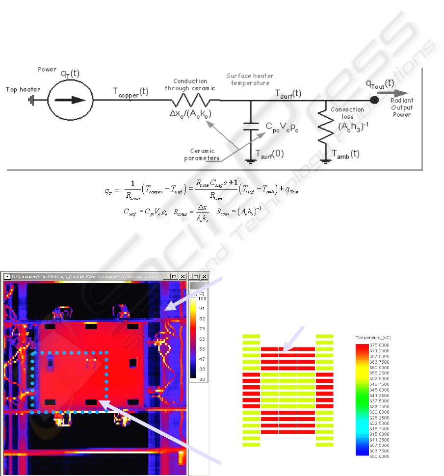
The view factor defines the relation W

between the

heat flux produced by heating element i and the

radiative power absorbed by sheet zone j in equation

(1). This heat flux can be measured by a sensor as

has been demonstrated by Kumar (2005).

Welement

[]

= Wzone

[]

(1)

The left part of Figure 5 presents the temperature

map at the exit of the oven with the holes provided

for the heat flux sensors appearing in black. In this

picture the heat flux sensor was located at the center.

2.1.3 Energy Absorption by the Sheet

(Process Parameter)

Energy is transferred throughout the sheet by two

mechanisms: conduction from the surface and

radiation absorption. The two related material

parameters are the conductivity and the absorptivity

of the material, respectively. A major source of

uncertainty in the process stems from the fact that

these parameters can vary widely from batch to

batch, especially for absorptivity which can vary

enormously when the colorant supplier is changed

for example, and techniques were designed to detect

on-line variations in these parameters.

Figure 4: Heating element transfer function (Gauthier et al., 2006).

4 Fluxmeter positions studied

Gains matrix is identified by generating a 50C

variation from uniform 350C heater map

Simulation run directly from scanning

thermometer output and then tuned from the

flux and tem

erature measurements

Figure 5: Sheet heat map at the exit of oven and heating element array (Girard et al., 2005).

ENERGY MODEL BASED CONTROL FOR FORMING PROCESSES

In general, the temperature increase in a given zone

of the sheet and at a given depth for a steady heat

flux can be represented with very good precision by

the following empiric equation where θ is

temperature, t is time, and d is depth into the sheet

(Girard et al., 2005).

(2)

Using this equation means that we know the

constant heat flux that is required to heat the sheet to

a given temperature θ

at time t and depth d. The

constants a1, a2 and a3 are determined by the fit

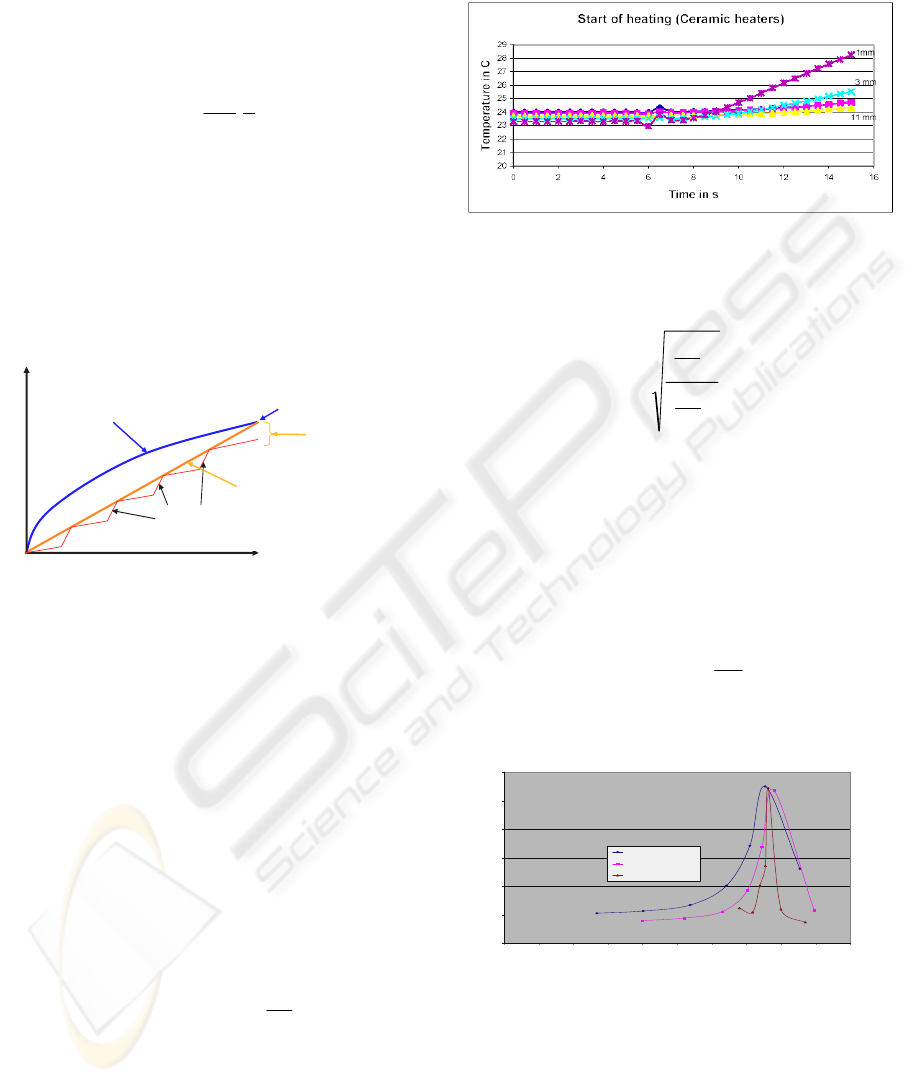
with modelled data. Figure 6 presents the variation

of temperature for a steady heat flux (constant

heating element temperature) together with the

repeated adjustments needed by a PID controller.

Repeated adjustments for ramping

PID control with major final error

Time

atu

Temperature

To be realized at time t

FluxSteadyfor

PID Ramp

Final error

for PID ramp

Figure 6: PID ramp and model based temperature control

comparison. Model based control achieves final state

temperature with more accuracy and less adjustment

during heating.

2.1.4 Absorptivity (Material Parameter)

The measurement of the start of heating for a virgin

(i.e., not colored) high density polyethylene thick

sheet reveals that even at a depth of 11 mm the

material temperature starts to increase nearly

immediately with the start of radiative sheet heating

(Figure 7). Since conduction heating requires several

minutes to get to this depth, the only heating

mechanism that can allow for such a behavior is

radiation absorption.

The energy absorbed, q

absn

, in layer ‘n’ contributes to

the internal temperature change according to:

cqF

pabsn

ραα

∂

==− )1(

(3)

where F

is the heat flux at the surface of the sheet,

α is the absorptivity, ρ is the sheet density, c

is the

heat capacity, ∂T is the sheet temperature difference

during time ∂τ, and x is the n

layer thickness. From

equation (4) (Kumar, 2005), the absorptivity α can

be calculated from the slopes of the temperature

increase measured at layers 3 and 1.

Figure 7: An enlargement of the start of sheet heating

(Girard et al., 2005). The data show the temperature

increase with time at different depths in a plastic sheet

being heated from the surface.

)(

∂

−=

(4)

2.1.5 Heat Capacity (Material Parameter)

The heat capacity C

is evaluated during the cooling

phase from the cooling rate with a given heat

transfer coefficient at the sheet surface (Figure 8)

(Zhang, 2004). The total energy, q

tot

, can also be

determined from the heat transfer coefficient as

follows

tot

≅ q

conv

≅

(5)

where the energy from the heating elements hitting

the sheet is the convection energy, q

conv

500

1000

1500

2000

2500

3000

50 60 70 80 90 100 1 10 120 130 1 40 150

Tem perature(C)

Heat Capacity(J/kg C)

1.5 m/s fan speed

0.55 m/s fan speed

0.005 m/s fan speed

Figure 8: Experimental heat capacity curves determined by

different cooling rates obtained on-line by varying fan

speed (bottom heating of the sheet at 280°C).

Please note in Figure 8 that different cooling rates

predict mostly the same heat capacity, and that the

shape of this peak is directly related to the level of

crystallinity of the material.

t,d

()

⎛

⎝

⎜

⎞

⎠

⎟

⎛

⎝

⎜

⎞

⎠

⎟

exp

ICINCO 2008 - International Conference on Informatics in Control, Automation and Robotics

2.1.6 Elastic Modulus (Material Parameter)

During the re-heat phase of the thermoforming

process the frozen in stresses induced in the material

during the calendering process are relaxed. This

results in anisotropic shrinkage of the sheet that

causes variation of the sag in the heating oven. The

forming of the shrunk sheet results in variations of

the final thickness of the produced part. Also, the

sag during heating must be adequately controlled

since it can result in catastrophic variations in the

distance from the sheet to the heating elements.

The elastic modulus, E, and level of frozen-in

stresses are the main predictors for sag and

shrinkage during the heating phase of the

thermoforming process.

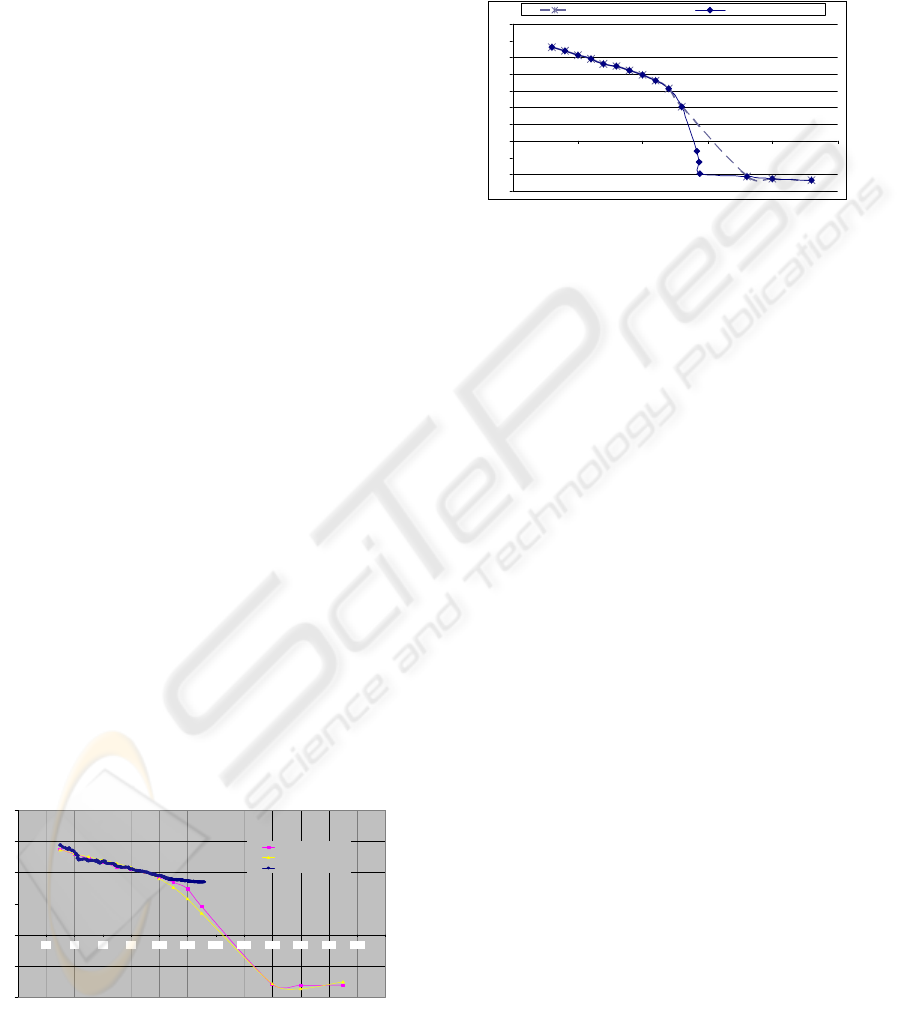
It is however difficult to get adequate data for

process control and simulation purposes given the

variability of sheet material properties from batch to

batch and the fact that the variation of E is difficult

to evaluate by the usual techniques in the vicinity of

the melting point of the material where the

experimental data reveals a very sharp inflection

point related to the phase change of the material.

Since forming takes place in this temperature region

simulation models are quite deficient in this crucial

area.

To address these issues an on-line identification

technique was developed that uses two different

steps of the blow forming process (Bahadoran,

2005). The low temperature variation of the elastic

modulus is identified from the development of the

sag at the entry in the oven (Figure 9) allowing for a

better evaluation of E near the melting point.

However, an existing forming mould can be used to

produce a bubble on-line on the actual forming

machine, and the value of the elastic modulus is

characterized near the transition point of the material

from the variation of the bubble and the blow

pressure (Figure 10) (Bahadoran, 2005).

-2

-1

20 40 60 80 100 120 140 160 180 200 220 240 260

Temperature (C)

Log

(E)

E(T)

Fit_3D

E(T) from Sag

Figure 9: Experimental data obtained on-line showing the

variation of the elasticity modulus with temperature at

lower temperatures.

This provides a much better definition of the ‘elbow’

zone of E versus temperature. This technique

requires minimal additional instrumentation to an

existing machine. Also most any existing mould can

be used for this purpose.

-1.5

-1

-0.5

0.5

1.5

2.5

3.5

0 50 100 150 200 250

Temp.(°C)

Log E (MP)

Without Bubble Data Bubble Data Added

Figure 10: Experimental data obtained on-line showing the

variation of the elasticity modulus with temperature,

particularly near the melting point.

2.2 Forming Energy during the

Forming Phase

Referring to Figure 2, after the sheet has been heated

the forming process begins at point 1 by applying a

constant pressure from one side of the sheet to be

formed. The material starts taking a more or less

spherical shape and its thickness diminishes. As the

shear rate of the material increases, the viscosity of

the material drops. Since the input pressure remains

relatively constant, this results in an unstable and

very fast evolution towards point 2 when the shear

rate rises above a triggering level.

After this point, the forming process can behave

either in a stable or an unstable manner depending

on the type of thermoplastic.

• If the material is shear strengthening,

deformation under constant pressure is

relatively easy to control since it will be

mostly spherical and bounded at point 3 and

then revert back to a stable behaviour. Also,

since the deformation is self-stabilizing the

shape of deformation tends to be spherical.

This is how the blow moulding of PET

(polyethylene terephthalate) materials is

controlled, for example.

• If the material is shear thinning, a pressure

control scheme results in the sheet being

ripped apart in an explosive manner. Also, any

deformation that starts at a given location

typically ‘grows‘ in a random direction and

pattern. In this case, the forming process needs

to be either bound geometrically by a mould

or by the flow rate that is applied to ‘blow’ the

sheet.

ENERGY MODEL BASED CONTROL FOR FORMING PROCESSES

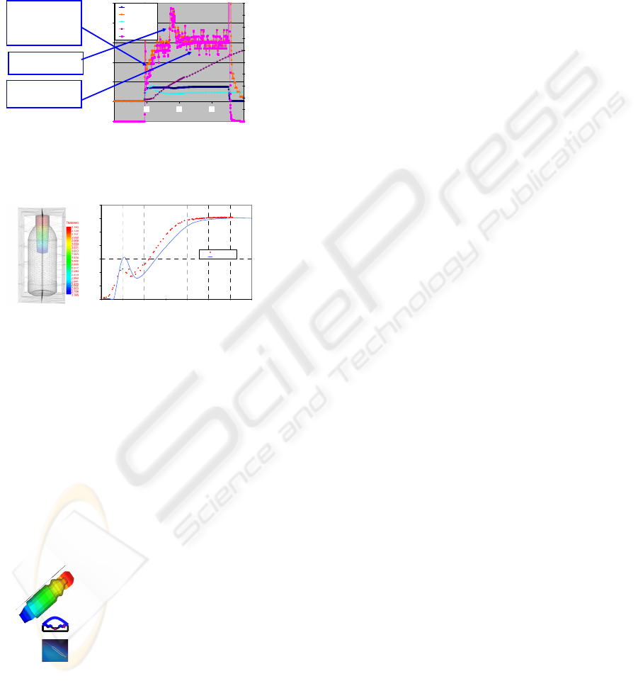
Figure 11 presents how the volume and pressure

develop for the free blow (forming without a mould)

of a PET bottle. It can be seen that the formed part

starts by expanding in a smooth manner in phase 1

until it suddenly expands very rapidly in phase 2.

Since PET is shear strengthening it will then

consolidate in phase 3.

-5.00E+01

0.00E+00

5.00E+01

1.00E+02

1.50E+02

2.00E+02

2.50E+02

10 15 20 25 30

Time in s

Pressure in PSI

0.00E+00

5.00E-03

1.00E-02

1.50E-02

2.00E-02

2.50E-02

3.00E-02

3.50E-02

4.00E-02

4.50E-02

5.00E-02

Pressure PSI

Flow Rate *100

Pred. P PSI

Pred. Vol. M^3

Power

Phase 2: Part expansion

takes place

Phase1: Pressure

increases until it

overcomes

material

resistance

Phase 3: Material

reaches

consolidation

Figure 11: Measuring the pressure/volume relationship for

free blow (blowing without a mould) of a PET bottle

0.00

0.10

0.20

0.30

0.40

0.50

0.60

0.70

0 0.10.20.30.40.50.60.7

Blowing Time (Sec)

Pressure (MPa)

Measured

Predicted

Initial Volume = 0.026 L

Final Volume = 0.473 L

Figure 12: Predicted and measured pressure with the

forming

simulation approach (PET bottle in mould).

It is easy to measure on-line the pressure and the

flow rate for these processes, and recent

developments show that simulations based on the

forming energy are much more accurate than those

relating constitutive equations to initial temperature

and pressure conditions on the sheet (Figure 12)

(Mir et al., 2007). Also, minimizing the amount of

energy required by the process, which allows for the

use of smaller machines, is often one of the

objectives of the control system.

Blowing of PET bottle:

Q is high and V is low

Triggering point: strain rate goes above given level

Bubble forming, gas tank:

Q is low and volume is high

Triggering point not reached

Angioplasty balloon forming:

Q is extremely low and volume is low

Triggering point: thickness goes below given level

Figure 13: Development of volume flow Q and volume V

for some thermoforming processes.

It must be noted that the start and development of

phase 2 (Figure 11) is not predicted by the usual

techniques, but that it poses no problem with the

forming

approach (Figure 12). Also, the ‘trigger’

point (Figure 13) that starts the expansion phase is

not predicted at all with the regular modeling

approach.

3 CONTROL TECHNIQUES

PRESENTLY USED FOR

THERMOFORMING

The control techniques presently used are typically

based on indirect sheet temperature control and a

forming pressure that is set to a constant value.

These techniques have major drawbacks.

• They do not directly control the main

parameters of the process.

• They do not monitor and do not control

adequately the primary process variables. This

is especially true of the forming pressure since

it is only regulated at the entry of the mould,

and often very imprecisely.

• They do not identify nor take into account the

switch point from stability to instability.

• During the unstable phases of the process,

minor variations in the input variables of the

process can develop into chaotic variations in

the end process. These variations are presently

not detected and are only taken into account in

the system indirectly. They can be:

o material properties that vary from

batch to batch,

o environmental variations such as

ambient temperature or air flow, and

o variations in machine parameters such

as heating elements output or line

pressure.

• Present temperature controllers, such as

implemented by MAGI Control (Montreal,

Canada), use a PID controller to track a ramp

that is calculated from the θ

temperature to be

realized. Figure 5 presents a comparison of the

model based and PID ramping approach based

on the results obtained by MAGI Control.

• These process uncertainties are compounded

by the new ‘designer’ materials that typically

have a very narrow processing window, and

also by the very tight dimensional

requirements that are required of technical

parts

ICINCO 2008 - International Conference on Informatics in Control, Automation and Robotics

It can be seen that PID control based on a ramp

requires repeated adjustments during the heating

phase and ends up with a considerable final error.

Model based control however only requires the

adjustment of the heat flux by integration of the

heating curve, which achieves much smoother

control and better final temperature precision.

4 MODEL BASED CONTROL

SYSTEM

In place of PID control, we are proposing to use a

model based control system that is continuously

tuned and based on on-line identification of the main

parameters of the forming processes that were

presented in Section 2. This ‘tuning’ is achieved by

intelligent agents as defined by (Weiss, 1999):

“Agents are autonomous, computational entities

which sense their environment either by physical or

virtual sensors, and then initiate actions by actuators

and/or by communicating with other agents.” In our

case each agent is a fast response routine that

monitors a specific aspect of the process, for

example, the variation of the specific heat of the

material. If this variation is

above a specific level,

the agent contacts the main system so that the

process parameters are adjusted to reflect the

change.

4.1 General Specifications of the

System

Error

Recovery

Module

Physical Layer

Database

Model

Control Module

Process model

Module

Diagnosis

Module

Figure 14: General architecture of the model based control

system.

4.1.1 Objective

• Implementation of a generalized controller

that is based on a model of the process to be

controlled and that updates and tunes the

process model in real time.

4.1.2 Inputs

• Real time measurements of the process and

equipment data.

• Results of quality control.

• Process submodels implemented as intelligent

agents that identify and track parameters and

that calculate process state parameters.

4.1.3 Outputs

• Updated control model with control

parameters that are sent to the forming

process.

• Process and material parameters are estimated

during part manufacture and are updated after

each part is made.

• Diagnostics of the process are executed during

part manufacture.

4.2 Main Control Module

4.2.1 Simulator Agent

The first step for the creation of a model based

control system using intelligent agents is to build an

accurate process model and simulator. The process

model identifies critical state variables and the

simulator predicts the parameter adjustments

required for the desired outcome from the state

variable history. A finite element simulation of the

thermoforming process based on the E

forming

energy

in equation (3) is very easy to correlate to real time

machine measurements of the flow rate and

pressure. This simulation typically requires:

• the geometric description of the part, machine

and moulds,

• a material database for the rheological and

physical properties of materials, and

• the processing parameters for the part, often

called recipe by the manufacturer.

Also, two main challenges need to be addressed for

adequate control.

• Inaccessible internal sheet temperatures need

to be controlled precisely within the forming

window for part quality.

• The execution time frames of the different

agents need to be adjusted and synchronized.

ENERGY MODEL BASED CONTROL FOR FORMING PROCESSES

4.2.2 Simulation of a Virtual Sensor

The tuned simulation can function as a virtual

sensor, also called a soft sensor. The integrated

history of the sheet surface temperature as measured

directly by infrared sensors with the heat transfer

simulation to predict the sheet internal temperature

and to indicate the time required for adequate sheet

heating inside the oven.

One of the main outputs of the simulation is the

predicted heating curve for the material for a

constant heat flux (Equation (2)) shown in Figure 6.

From this, the system can control the heat flux by

controlling the heating element input power, which

results in a given temperature at a given depth at

time t in the material.

4.2.3 Adjusting the Time Frames of the

Different Modules

Unfortunately, the time frame of such a simulation is

orders of magnitude greater than what is needed to

control the thermoforming process in real time. This

problem is solved by generating the sensitivity

matrix of the simulation every time the simulation is

updated. For example, the heat flux in equation (3)

can be generated from the tuned simulation.

Equations (2, 3) are used to predict the sheet

temperatures at different depths for different sheet

zones for the time sequenced trajectories of the

heating element energy input allowing for heat flux

control as shown in Figure 5.

Since the simulation is reasonably accurate, the

control system only needs to apply the updated

parameters in the vicinity of the initial prediction for

the calculated operating point, which allows the use

of linear interpolations to adjust the operating point

as required, thus achieving a very fast response time.

4.3 Agent based Control

An intelligent agent based system is a loosely

coupled network of problem solving entities (agents)

that work together to find the answer to problems

that are beyond the individual capabilities or

knowledge of each entity (Florez-Mendez, 1999).

An agent based system was chosen for model based

control since it can deal well with multiple

submodels and data streams, and can cope with

submodels that are very different in size and that

operate on dissimilar time scales. These features

make agent technology especially suited for building

control systems based on models of processes,

where the processes are very complex and many

process and material parameters are dynamic.

All agents in the architecture operate

independently and asynchronously. The control

agent acquires sensor data from the physical layer

and sends control parameters as they become

available. Similarly, the process agents retrieve

sensor data and calculate state variables. The

retrieval of sensor data and the calculation of state

variables are interrupt driven based on detected

variations from previous states; thus, calculations are

only launched when needed and with the best

information available. This design minimizes control

cycle time while allowing data to flow

asynchronously and implements just in time delivery

of the different data streams, while still setting

control parameters with complex, but validated

parameters. The result is that during a short

production period certain parameters are updated

infrequently. This is not a problem, since they do not

highly impact the operating point of the process.

This architecture allows many processes to be

controlled in-cycle, i.e., while a part is being made

so that near perfect parts can be made every time. If

the process is very fast or parameters cannot be

measured during part manufacture, cycle-to-cycle

control can be done, i.e., parameters measured

during or after a part is being made are used to

control the next part being manufactured.

Control can be done with a single processor, if

the amount of computation is small. Nevertheless,

for a complex process like thermoforming, the

amount of calculation for process models tends to be

large and distributed over different time frames;

therefore, multiple processors may be required

depending on the complexity of the heating process.

With multiple processors, the control system can

dynamically allocate the execution of different

agents to different processors. Due to the

asynchronous operation of the architecture,

processes can be optimally controlled for submodel

execution times from milliseconds to hours.

5 PARAMETERS IDENTIFIED

ON-LINE

If the agent in charge decides that the drift or

variation of the parameter warrants an adjustment of

the simulator, parameters are changed and the

simulation is then re-run and the control models

regenerated. For the thermoforming process, the

following parameters are continuously monitored in

real time.

ICINCO 2008 - International Conference on Informatics in Control, Automation and Robotics

• absorptivity

• heat capacity

• elastic modulus of the material.

Machine parameters that are monitored on-line

are:

• input power of the heating elements

• surface temperature of the sheet in the oven

• forming pressure

• forming energy flow rate

• mould temperature.

Ambient parameters that are monitored on-line

are:

• ambient temperature

• oven air temperature

• air velocity in the oven during sheet heating

• air velocity during the cooling phase after

forming.

6 DIAGNOSTIC SYSTEM

A diagnosis module monitors the behaviour of the

process during control. The agents that monitor the

system act to detect any abnormal behaviour based

on previously accumulated know-how about the

process. They then either try to correct the anomaly

(error recovery agent) or stop the machine in the

case of a non-recoverable error. In all cases the

operator is advised. Diagnostics and error recovery

operate independently and asynchronously with

respect to the process and control modules. More

detail is given in Albadawi et al. (2006).

7 CONCLUSIONS

The model based control system proposed here for

the thermoforming process:

• uses the energy required as the main control

variable, allowing for easy energy

minimization,

• can target a specific temperature at a specific

depth and a specific time by adjusting a single

state parameter,

• can predict the switch from steady to unsteady

state in the process,

• can detect and adjust for a range of variations

of material and machine parameters,

• has a response time that is adequate for in-

cycle control, and

• inherently minimizes cycle time while

respecting the process and material limitations.

Agent technology is an excellent match for control

based on process models since it allows distributed

intelligence and decision making to be applied to the

control problem.

Subsystems for the control system have been

developed and a system is being built to test control

of an industrial thermoforming process.

REFERENCES

Ajersch, M., 2004. Modeling and real-time control of

sheet reheat phase in thermoforming. Master’s thesis,

Department of Electrical Engineering, McGill

University.

Albadawi, Z., Boulet, B., DiRaddo, R., Girard, P., Rail, A.

and Thomson, V., 2006. Agent-based control of

manufacturing processes. Int. J. Manufacturing

Research, 1(4) 466–481.

Bahadoran, 2005. Online characterization of viscoelastic

and stress-relaxation behavior in thermoforming.

Master’s thesis, Department of Mechanical

Engineering, McGill University.

Florez-Mendez, R., 1999. Toward a standardization of

multi-agent system frameworks. ACM Crossroad,

5(4), 18-24.

Gauthier, G., Ajersch, M., Boulet, B., Haurani, A., Girard,

P., DiRaddo, R., 2005. A New Absorption Based

Model for Sheet Reheat in Thermoforming, SPE

Annual Technical Conference, ANTEC, Boston,

Massachusetts.

Girard, P., Thomson, V., Boulet, B., DiRaddo, R.W.,

2005. Advanced in-cycle and cycle-to-cycle on-line

adaptive control for thermoforming of large

thermoplastic sheets. SAE World Congress, Detroit,

MI, USA.

Kumar, V., 2005. Estimation of absorptivity and heat flux

at the reheat phase of thermoforming process.

Master’s thesis, Department of Mechanical

Engineering, McGill University.

Mir, H., Benrabah, B., Thibault, F., 2007. The use of

elasto-visco-plastic material model coupled with

pressure-volume thermodynamic relationship to

simulate the stretch blow molding of polyethylene

terephthalate, Numiform, Porto, Portugal.

Weiss, G., 1999. Multiagent systems, MIT Press,

Cambridge, USA.

Zhang, Y., 2004. Generation of component libraries for

the thermoforming process using on-line

characterization. Master’s thesis, Department of

Mechanical Engineering, McGill University.

ENERGY MODEL BASED CONTROL FOR FORMING PROCESSES