
DISCRETE-EVENT SIMULATION OF A COMPLEX
INTERMODAL CONTAINER TERMINAL
A Case-Study of Standard Unloading/Loading Processes of Vessel Ships
Guido Maione
DEESD, Technical University of Bari, Viale del Turismo 8, I-74100, Taranto, Italy
Keywords: Container Terminals, Discrete-Event Systems, Simulation, Transport Systems.
Abstract: This paper analyzes the performance of a complex maritime intermodal container terminal. The aim is to
propose changes in the system resources or in handling procedures that guarantee better performance in
perturbed conditions. A discrete-event system simulation study shows that, in future conditions of increased
traffic volumes and reduced available stacking space, more internal transport vehicles, or appropriate
scheduling and routing policies, or an increased degree of automation would improve the performance.
1 INTRODUCTION
In an intermodal container terminal (CT) freight is
organized, stacked, handled and transported in
standard units of a typical container, which is called
TEU (Twenty Equivalent Unit) and which fits to
ships, trains and trucks that are built and work for it.
A maritime CT is usually managed to offer three
main services: a railway/road ‘export cycle’, when
TEUs arrive by trains/trucks and depart on vessel
ships; a railway/road ‘import cycle’, when TEUs
arrive on vessel ships and depart by trains/trucks; a
‘transshipment cycle’, when TEUs arrive on vessel
(feeder) ships and depart on feeder (vessel) ships.
The hub in Taranto is managed by a private
company (Taranto Container Terminal or TCT),
whose primary business is for transhipment, because
of the low quality of railway and road networks
connecting the hub to Italy and the rest of Europe.
The terminal receives ships to a quay and uses
yard blocks to stack full or empty TEUs. Imported
TEUs are unloaded, exported TEUs are loaded,
while in transshipped TEUs both processes occur.
Full TEUs may be imported, exported or
transshipped. Empty TEUs are unloaded from feeder
ships or arrive on trains or trucks; then they are
loaded on vessel ships. So, they are transhipped or
exported.
The typical activities executed by humans and
resources in a transshipment cycle are the following:
Unloading TEUs from ship by quay cranes;
Picking-up and transferring TEUs to a yard
block by trailers;
Picking-up and stacking TEUs in a yard block
by yard cranes;
Redistributing TEUs in yard blocks by yard
cranes and trailers;
Picking-up and transferring TEUs to ship by
yard cranes and trailers;
Loading on ship by quay cranes.
Managing these activities requires an optimized
use of equipment and human operators. Human
supervision is often required to control processes
concurring and competing for the limited number of
available resources. Moreover, efficiency is needed
for services in reduced time without excessive costs:
both the TCT needs to profitably use resources, and
ship companies aim at saving the berthing time/cost.
TCT is expecting a growth in freight volumes
and has recently expanded the yard. But no
investment was made on local land infrastructures.
Not much research was carried out on use of
information and communication technologies or new
control policies to improve efficiency, to the best of
the author knowledge. Improvements can be
achieved for TCT, which is very sensitive to
disturbances and parameter variations (sudden or big
increase of traffic volumes, reduction or
reorganization of yard, changes in berthing spaces,
different routing of trailers, faults and malfunctions).
Then, an intelligent control may guarantee
robustness and a quick reaction to parameter
variations. The aim here is to prove that current
171
Maione G. (2008).
DISCRETE-EVENT SIMULATION OF A COMPLEX INTERMODAL CONTAINER TERMINAL - A Case-Study of Standard Unloading/Loading Processes
of Vessel Ships.
In Proceedings of the Fifth International Conference on Informatics in Control, Automation and Robotics - SPSMC, pages 171-176
DOI: 10.5220/0001499801710176
Copyright
c
SciTePress

organization and control of the main unloading and
loading processes could be not efficient in future
operating conditions. Changing management of
operations is necessary to guarantee good
performance in perturbed conditions.
2 LITERATURE OVERVIEW
Managing a maritime CT is a complex task. Several
analytical models have been proposed as tool for the
simulation of terminals useful to an optimal design
and layout, organization, management and control.
Modelling CTs requires the simulation of many
operations that need coordination to minimize time
and costs. Determining the best management and
control policies is also important (Mastrolilli et al.,
1998). The main problems are: berth allocation;
loading and unloading of ships (crane assignment,
stowage planning); transfer of TEUs from ships to
yard and back; stacking operations; transfer to/from
other transport modes; workforce scheduling.
A thorough literature review on modelling
approaches is given in (Steenken et al., 2004). Two
main classes of modelling approaches can be
highlighted: microscopic and macroscopic methods
(Cantarella et al., 2006). Microscopic models are
generally based on discrete-event system simulation
that may include Petri Nets (Fischer and Kemper,
2000, Liu and Ioannou, 2002), object-oriented
(Bielli et al., 2006) and queuing networks theory
approaches (Legato and Mazza, 2001). Even if high
computational effort may be required, microscopic
simulation explicitly models all activities as well as
the whole system by considering the single TEUs as
entities. Then, it estimates performance as
consequence of different designs and/or
management scenarios.
Macroscopic modelling (de Luca et al., 2005) is
suitable for supporting strategic decisions, system
design and layout, investments on handling
equipment. A network-based approach is presented
in (Kozan, 2000) for optimising efficiency by using
a linear programming method.
3 DEVS MODELLING
A Discrete EVent System (DEVS) specification
technique (Zeigler et al., 2000) completely and
unambiguously represents and controls the terminal
processes.
Atomic dynamic DEVSs model both TEUs
flowing in the system and resources (cranes, trailers,
trucks) used to handle them. DEVSs interact by
transmitting outputs and receiving inputs, which are
all instantaneous events. Timed processes are
defined by a start-event and a stop-event.
For each DEVS, internal events are triggered by
internal mechanisms, external input events are
determined by other DEVSs, and external output
events are generated and directed to other entities.
A DEVS state is changed by an input or when
the time specified before an internal event elapses.
In the first case, an external transition function
determines the state next to the received input; in the
second case, an internal transition function gives the
state next to the internal event. The total state is q =
(s, e), where s is the sequential state and e is the time
elapsed since the last transition.
To summarize, each DEVS is represented as:
DEVS = < X, Y, S,
δ
in
t
,
δ
ex
t
,
λ
, ta >
(1)
where X is the set of inputs, Y is the set of outputs, S
is the set of sequential states,
δ
int
:S→S is the internal
transition function,
δ
ext
:Q×X→S is the external
transition function, Q={q=(s,e)|s∈S,0≤e≤ta(s)},
λ
:S→Y is the output function, ta:S→ℜ
0
+
is the time
advance function, with ℜ
0
+
set of positive real
numbers with 0 included.
The network of DEVS atomic models is used as
a platform for simulating the TCT dynamics. Details
are omitted here for sake of space.
4 SIMULATION ANALYSIS
A simulation study is presented to analyse the
contemporaneous processes of unloading and
loading TEUs from and to a vessel ship.
The simulation model is based on the real TCT
equipment and operation times, which were
statistically observed during steady-state conditions.
The model was developed in a discrete-event
environment by using Arena
®
(Kelton et al., 1998).
4.1 Experimental Setup
The data used to set up the simulation experiments
refer to the observations recorded during year 2004,
when TCT achieved the maximum productivity
(Table 1). About 14% of TEUs flew through
railway/road transport modes. The numbers of
full/empty TEUs are divided as in Table 2.
ICINCO 2008 - International Conference on Informatics in Control, Automation and Robotics
172
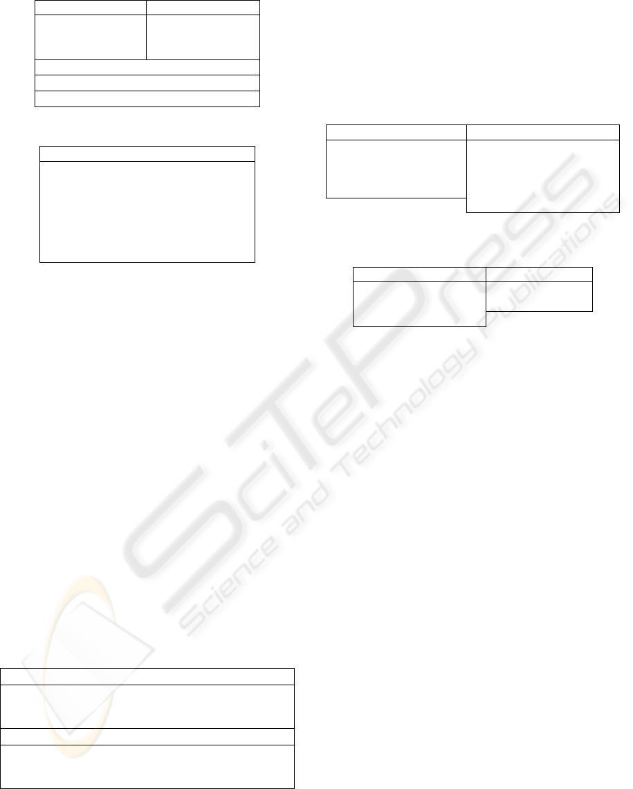
Table 1: Loaded/unloaded TEUs in TCT (2004).
Loaded TEUs Unloaded TEUs
Full
273224
Full
285488
Empty 108172 Empty 96434
Total TL 381396 Total TD 381922
Total T = TL+TD = 763318
TEUs on railway 44486 ≅ 5.8% of T
TEUs on road 64648 ≅ 8.5% of T
Table 2: Flows of containers in TCT (2004).
Containers (Cycle) No.
Full, from vessel to feeder x
Full, from feeder to vessel y
Full, from vessel to train/truck t
Full, from train/truck to vessel z
Empty, from feeder to blocks r
Empty, from train/truck to blocks h
Empty, from blocks to vessel q
Then, we may establish the following relations:
x + y + z = 273224 (2)
q = 108172 (3)
x + y + t = 285488 (4)
r = 96434 (5)
t + z + h = 113134 (6)
r + h = q (7)
where (7) is due to the assumption that no empty
TEU is accumulated and left in the yard blocks.
Then, it is easy to find: x+y = 228658, t = 56830,
z = 44566, r = 96434, h = 11738, q = 108172. The
TEUs separately handled by vessel and feeder ships
were estimated in the ranges in Table 3, because x
and y were assumed between 0 and 228658. Then,
the average number of TEUs handled by vessel (avs)
or feeder ships (afs) was determined by assuming
traffic volumes of 346 vessel and 570 feeder ships in
year 2004. These assumptions were based on the
traffic data available for year 2003 and on the 15.9%
increase in traffic (then in number of ships) in 2004.
Table 3: Containers handled by ships.
Vessels TEUs Est. Range
avs
Unload. x+t [56830,285488] [164,825]
Loaded y+z+q [152738,381396] [441,1102]
Total x+t+y+z+q 438226 1266
Feeders TEUs Est. Range
afs
Unload. y+r [96434,325092] [169,570]
Loaded x [0,228658] [0,401]
Total y+r+x 325092 570
If x = y = 114329, then the flows indicated by
Tables 4 and 5 are obtained, which were used to set-
up the simulation tests. Flows of TEUs from vessel
ships to land are in a ratio 8 to 6 between road and
railway modes, as observed in 2004. Unloaded and
loaded TEUs are 39% and 61% of the total for
vessel ships, 65% and 35% for feeder ships.
Table 4: Containers unloaded (U) and loaded (L) by vessel
ships (F = feeder ships, TA = trains, TU = trucks, E =
blocks for empty TEUs).
U No. (%) L No. (%)
To F 114329 (66.80) From F 114329 (42.81)
To TA 24356 (14.23) From E 108172 (40.50)
To TU 32474 (18.97) From TA 19100 (7.15)
Total 171159 (100) From TU 25466 (9.54)
Total 267067 (100)
Table 5: Containers unloaded (U) and loaded (L) by feeder
ships (V = vessel ships, E = blocks for empty TEUs).
U No. (%) L No.
To V 114329 (54.24) From V 114329
To E 96434 (45.76) Total 114329
Total 210763 (100)
4.2 Simulation Assumptions
Simulation is based on the following assumptions:
Only 1 vessel ship is berthed, full TEUs are
unloaded, full and empty TEUs are loaded;
1300 TEUs are handled; 508 (39%) are
unloaded, 792 (61%) are loaded, according to
the percentage partitions shown in Table 4;
The average values of handled TEUs in Table 3
is used, because information about daily
movement or ship size was not available;
Simulation is limited by the time necessary to
end the unloading and loading processes;
Transfers from/to the railway connection or the
truck gate, are not considered;
Operations length and distances travelled are
measured in minutes and meters, respectively.
The model considers four quay cranes: QC1 and
QC2 are for unloading, QC3 and QC4 for loading.
Then, unloaded TEUs are stowed in ship sections
different from those reserved for loaded TEUs, so
that the processes are parallel. Sometimes cranes
sequentially unload and load TEUs, depending on
the stowage plan and on the destinations of TEUs.
A quay crane unloads/loads two TEUs on/from a
trailer in eight steps (Table 6): S1) picking the first
TEU from ship/trailer; S2) moving the crane with
first TEU towards the trailer/ship; S3) releasing the
first TEU on the trailer/ship; S4) moving the crane
back to the ship/trailer; S5) picking the second TEU
from ship/trailer; S6) moving the crane with second
DISCRETE-EVENT SIMULATION OF A COMPLEX INTERMODAL CONTAINER TERMINAL - A Case-Study of
Standard Unloading/Loading Processes of Vessel Ships
173
TEU to the trailer/ship; S7) releasing the second
TEU; S8) moving the crane back to the ship/trailer.
Table 6: Operation cycle of quay cranes.
Step Duration
S1 Tria(0.4375,0.5,0.75)
S2 0.333
S3 Tria(0.4375,0.5,0.75)
S4 0.667
S5 Tria(0.4375,0.5,0.75)
S6 0.333
S7 Tria(0.4375,0.5,0.75)
S8 0.667
The triangular distribution is used because only
the estimates of the minimum, most likely and
maximum values (shown in this order) of the
processing times are known. Simple translational
return steps last longer (twice) than transfer steps
because the crane is more unstable without TEUs.
Five trailers serve each quay crane. Each set of
five trailers is indicated with a unique symbol: TR1,
TR2, TR3, TR4 are associated to QC1, QC2, QC3,
QC4, respectively. Each trailer always transports
two TEUs, with a speed of 300 m/minutes (400
m/minutes when travelling unloaded). The closest
trailer is selected for a task between ship and yard.
Before being loaded, exported and transshipped
TEUs are stacked in blocks close to the quay area,
while imported TEUs are stacked in blocks close to
the land connections. Only one yard crane works on
each block for unloaded TEUs from ships: YC1
serves transhipped TEUs; YC2/YC3 serves exported
TEUs. Two yard cranes (YC4 and YC5 or YC6 and
YC7) work for each block for TEUs to be loaded:
YC4 serves empty TEUs, YC5 serves full TEUs;
YC6 and YC7 serve full TEUs. YC7 has priority
with respect to YC6 because it is closer to the quay.
TEUs picked by YC4 and YC5 are loaded by QC3,
those picked by YC6 and YC7 are loaded by QC4.
A yard crane unloads/loads two TEUs in/from a
yard block from/to a trailer in eight steps (Table 7).
Table 7: Operation cycle of yard cranes.
Step Duration
S1 Tria(0.125,0.375,0.625)
S2 0.25
S3 Tria(0.125,0.375,0.625)
S4 0.5
S5 Tria(0.125,0.375,0.625)
S6 0.25
S7 Tria(0.125,0.375,0.625)
S8 0.5
A typical and important performance index is the
Ship Turn-around Time (STT), the average time
spent by a berthed ship to unload and load TEUs.
STT is measured between ship arrival and departure.
Minimizing STT is the main objective of every
terminal management. An empiric relation to
calculate the minimum STT value is:
STT
min
= nc / (ct × nqc)
(8)
where nc is the number of unloaded/loaded TEUs, ct
is the cycle time (the number of moves/hour of a
quay crane), and nqc is the number of quay cranes.
Equation (8) gives a reference for the terminal
productivity. Namely, it does not consider the
dependence of ct on nqc, due to the interaction
between nqc and the handling capacity in the limited
quay space, and the effects of internal transfers.
Figure 1 gives the STT when nc = 3400 and ct = 42
hours
-1
. Equation (8) can also be used to estimate the
necessary nqc to achieve a desired STT.
Figure 1: STT as function of nqc.
Assuming the most likely value ct = 30 hours
-1
, if
nc
u
= 508 and nc
l
= 792 are the unloaded and loaded
TEUs, and if nqc
u
= nqc
l
= 2 are the cranes used for
the two processes, then a reference limit for STT is:
STT
min
= max{ nc
u
/(ct×nqc
u
); nc
l
/(ct×nqc
l
)}
= max{8.5; 13.2} = 13.2 hours.
(9)
Finally, note that performance is affected by the
partial automation of processes, the humans’
cooperation, the non-optimal ship distribution of
TEUs and weather conditions.
4.3 Simulation Results
Ten simulation runs were executed, using different
seeds for generating random variables, in order to
obtain sufficient results for a statistical evaluation.
Each run was terminated after 1300 unloaded and
ICINCO 2008 - International Conference on Informatics in Control, Automation and Robotics
174
loaded TEUs. The system state was initialized at the
beginning of each run, to start from the same
condition. Statistics were also initialized to have
results independent on the data obtained from
precedent runs. Initializations guarantee statistically
independent and identically distributed replications
of the terminating simulation.
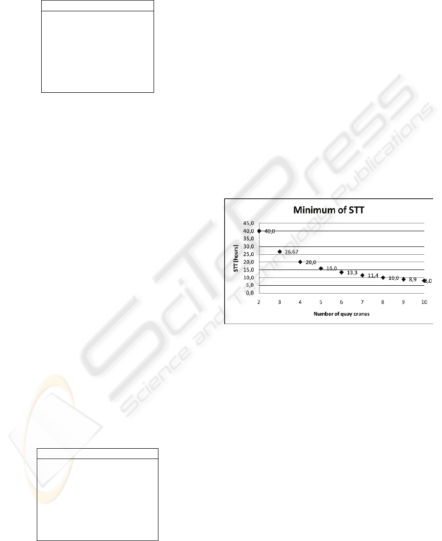
STT was measured at the end of each run (Figure
2). The minimum, maximum, and average values
were 891, 902, and 898, i.e. about 15 hours.
Figure 2: Measured STT in 10 simulation runs.
These results validate the model because:
They are below the real TCT performance,
because only 1 ship/day is served in standard
real operating conditions;
The measured values of STT are greater than
the lower theoretical limit established by (9).
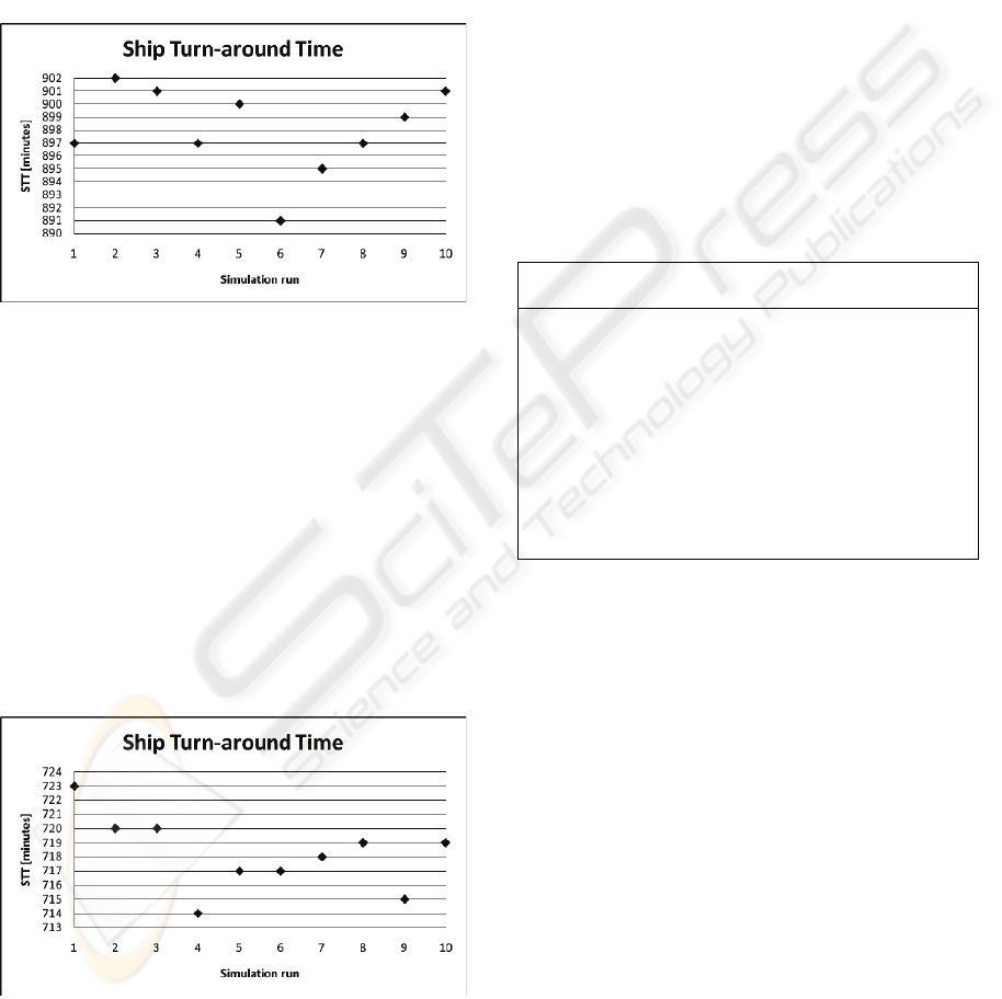
STT can be also measured for ships of different
capacity or with a distribution of TEUs different
from that in Table 4. If we let 1300 TEUs equally
distributed between the four quay cranes, we obtain
the results in Figure 3. The minimum, maximum and
average values of STT were, respectively, 714, 723,
and 718, that correspond to about 12 hours.
Figure 3: Measured STT in 10 simulation runs (TEUs
equally distributed between quay cranes).
Performance indices were measured for critical
resources like trailers and cranes: waiting times in
queue; number of entities in queue; resource
utilization. The associated statistics were: the
average value in 10 runs; the minimum average
value in a single run; the maximum average value in
a single run; the maximum value.
Table 8 shows the waiting times. For unloading
processes, TEUs may wait for the following busy
resources: a) TR1 or TR2, when being on QC1 or
QC2; b) YC1, YC2, YC3, when being on TR1 or
TR2. For loading processes, TEUs may wait for: a)
TR3, when being on YC4 used for empty TEUs; b)
TR3, when being on YC5 used for full TEUs (busy
resource TR3*); c) TR4, when being on YC6 used
for full TEUs; d) TR4, when being on YC7 used for
full TEUs (busy resource TR4*); e) QC3 or QC4,
when being on trailers TR3 or TR4.
Table 8: Waiting times in queue of busy resources.
Busy
Res.
Average Min.
Aver.
Max.
Aver.
Max.
Value
TR1 0.0788 0.00 0.1393 5.0002
TR2 0.0807 0.00 0.1613 4.7440
YC1 3.5193 2.5625 4.6946 17.7338
YC2 0.0612 0.00 0.1264 1.9246
YC3 0.0989 0.00 0.1965 2.0696
TR3 1.0662 1.0013 1.1135 6.8421
TR3* 28.4835 28.2937 28.6313 770.4400
TR4 5.1725 5.1165 5.2450 418.2100
TR4* 1.2628 1.21478 1.3079 7.8171
QC3 7.2326 7.0881 7.3267 10.5871
QC4 5.9521 5.8538 6.0713 10.2105
The average waiting times of TR1 and TR2 are
below 5 seconds, and then delays in unloading TEUs
due to the waiting of trailers below the quay cranes
can be neglected. So, more trailers are not necessary
for unloading in the simulated conditions. On the
contrary, the results for TR3, TR3*, TR4, TR4*
show that the loading process waits for long time
when yard cranes are used. Thus, at least one more
trailer should be used.
The large values for TR3* and TR4 were
obtained because of the priority given to empty with
respect to full TEUs, and because of the priority of
selecting the closest yard crane YC7 instead of YC6.
If we consider the interactions of trailers with
yard cranes during the unloading process, high
waiting times are observed for YC1 only, because
most of the unloaded TEUs were stacked in the
block served by YC1. More yard cranes would
speed-up the stacking process, but they are not
necessary since the number and speed of trailers is
DISCRETE-EVENT SIMULATION OF A COMPLEX INTERMODAL CONTAINER TERMINAL - A Case-Study of
Standard Unloading/Loading Processes of Vessel Ships
175

sufficient to guarantee fast and almost continuous
unloading operations by the quay cranes.
Long times are recorded for trailers when
waiting for quay cranes to load TEUs (more than 7
minutes for QC3 and about 6 minutes for QC4).
Then, one more trailer could help operations in the
yard area, because the maximum number of queued
trailers below a quay crane is three (see Table 9),
such that the other two are available for yard cranes.
Table 9 shows the results for the number of
entities in queue (the minimum value is always 0).
Table 10 shows the utilization of resources, i.e.
the percentage number of busy units or the
percentage busy time for single-unit resources (the
minimum is always 0, the maximum is always 1).
Table 9: Number of entities in queue of busy resources.
Busy
Res.
Average Min.
Aver.
Max.
Aver.
Max.
Value
TR1 0.0111 0.00 0.0199 1.0000
TR2 0.0114 0.00 0.0230 1.0000
YC1 0.6708 0.4637 0.9167 6.0000
YC2 0.0026 0.00 0.0062 1.0000
YC3 0.0056 0.00 0.0109 1.0000
TR3 0.2018 0.1911 0.2100 1.0000
TR3* 0.8882 0.8837 0.8906 1.0000
TR4 0.5703 0.5653 0.5770 1.0000
TR4* 0.1392 0.1339 0.1446 1.0000
QC3 1.5947 1.5753 1.6095 3.0000
QC4 1.3124 1.2990 1.3337 3.0000
Table 10: Utilization of resources.
Resource Average Min.
Aver.
Max.
Aver.
QC1 0.6104 0.6019 0.6218
QC2 0.6122 0.6036 0.6265
QC3 0.9919 0.9913 0.9926
QC4 0.9378 0.9324 0.9439
TR1 0.4818 0.4614 0.5013
TR2 0.4828 0.4660 0.5049
TR3 0.9897 0.9890 0.9899
TR4 0.9360 0.9307 0.9425
YC1 0.5712 0.5302 0.5970
YC2 0.1150 0.0892 0.1692
YC3 0.1617 0.1055 0.1812
YC4 0.8642 0.8612 0.8724
YC5 0.9825 0.9818 0.9831
Results for quay cranes indicate that unloading
with QC1 and QC2 terminates before loading with
QC3 and QC4. QC3 is used more than QC4 because
of the high number of empty TEUs. Considerations
about yard cranes are similar. Trailers TR1 and TR2
complete their tasks much earlier than TR3 and TR4,
which are practically always busy. Then, the
transport processes could benefit from more trailers.
5 CONCLUSIONS
This paper presents simulates a maritime terminal
container (TCT) in standard operating conditions.
Results prove the benefit from new control strategies
different from those currently used. A new control
approach could reduce terminal operating cycles in
standard and, above all, in perturbed operating
conditions.
REFERENCES
Bielli, M., Boulmakoul, A., Rida, M., 2006. Object
oriented model for container terminal distributed
simulation. European Journal of Operational
Research, Vol. 175, No. 3, pp. 1731-1751.
Cantarella, G.E., Cartenì, A., de Luca, S., 2006. A
comparison of macroscopic and microscopic
approaches for simulating container terminal
operations. In Proc. of EWGT2006 Joint conference,
Bari, Italy, 27-29 Sept. 2006.
de Luca, S., Cantarella, G.E., Cartenì, A., 2005. A
macroscopic model of a container terminal based on
diachronic networks. In Proc. Second Workshop on
the Schedule-Based Approach in Dynamic Transit
Modelling, Ischia, Naples, Italy, 29-30 May 2005.
Fischer, M., Kemper, P., 2000. Modeling and Analysis of
a Freight Terminal with Stochastic Petri Nets. In Proc.
of 9th IFAC Int. Symp. Control in Transp. Systems,
Braunschweig, Germany, vol. 2, pp. 195-200.
Kelton, W.D., Sadowski, R.P., Sadowski, D.A., 1998.
Simulation with Arena, McGraw Hill, New York.
Kozan, E., 2000. Optimising container transfers at
multimodal terminals. Mathematical and Computer
Modelling, Vol. 31, No. 10-12, pp. 235-243.
Legato, P., Mazza, R.M., Sept. 2001. Berth planning and
resources optimisation at a container terminal via
discrete event simulation. European Journal of
Operational Research, Vol. 133, No. 3, pp. 537-547.
Liu, C.I., Ioannou, P.A., 2002. Petri Net Modeling and
Analysis of Automated Container Terminal Using
Automated Guided Vehicle Systems. Transportation
Research Record, No. 1782, pp. 73-83.
Mastrolilli, M., Fornara, N., Gambardella, L.M., Rizzoli,
A.E., Zaffalon, M., 1998. Simulation for policy
evaluation, planning and decision support in an
intermodal container terminal. In Proc. Int. Workshop
Modeling and Simulation within a Maritime
Environment, Riga, Latvia, 6-8 Sept. 1998, pp. 33-38.
Steenken, D., Voss, S., Stahlbock, R., 2004. Container
terminal operation and operations research - a
classification and literature review. OR Spectrum, 26,
pp. 3-49.
Zeigler, B.P., Praehofer, H., Kim, T.G., 2000. Theory of
Modelling and Simulation, Academic Press. New
York, 2
nd
ed..
ICINCO 2008 - International Conference on Informatics in Control, Automation and Robotics
176
