TORQUE CONTROL WITH RECURRENT NEURAL NETWORKS
Guillaume Jouffroy
Artificial Intelligence Laboratory, University Paris 8, France
Keywords:
Joint constraint method, oscillatory recurrent neural network, generalized teacher forcing, feedback, adaptive
systems.
Abstract:
In the robotics field, a lot of attention is given to the complexity of the mechanics and particularly to the
number of degrees of freedom. Also, the oscillatory recurrent neural network architecture is only considered
as a black box, which prevents from carefully studying the interesting features of the network’s dynamics. In
this paper we describe a generalized teacher forcing algorithm, and we build a default oscillatory recurrent
neural network controller for a vehicle of one degree of freedom. We then build a feedback system as a
constraint method for the joint. We show that with the default oscillatory controller the vehicle can however
behave correctly, even in its transient time from standing to moving, and is robust to the oscillatory controller’s
own transient period and its initial conditions. We finally discuss how the default oscillator can be modified,
thus reducing the local feedback adaptation amplitude.
1 INTRODUCTION
Central Pattern Generators (CPG) are biological pe-
riodic oscillatory neural networks responsible for a
wide range of rhythmic functions. They can be made
of endogeneous oscillatory neurons connected to non
oscillatory ones or from the sole interaction between
non oscillatory neurons.
Particularly, they are a great source of inspiration
in the robotics field, for the control of joints in loco-
motion. In general, an oscillatory network controls a
joint angle in both directions, and the phase relation-
ships needed between all joints arise from the cou-
pling between the different networks.
The needed parameters for an artificial Recurrent
Neural Network (RNN) to have a periodic oscillatory
behavior cannot be measured experimentally. This
network is most of the time a relatively simplified
model of its biological counterpart when available.
Only clinical temporal data of joints kinetics and
kinematics can be of use, where however it is difficult
to isolate the real control of a particular joint from the
influence of the others.
In the case of non endogeneous oscillatory neu-
rons, in the litterature, parameters are thus mainly
determined empirically or with genetic algorithms
(Buono and M.Golubitsky, 2001), (Ghigliazza and
P.Holmes, 2004), (Ishiguro et al., 2000), (Kamimura
et al., 2003), (Taga, 1994), (Ijspeert, 2001), compara-
tively to relatively few learning methods (Mori et al.,
2004), (Tsung and Cottrell, 1993), (Weiss, 1997).
Though this is useful with large networks in complex
mechanical models, there are two drawbacks. It is
very difficult in general to isolate the resulting dynam-
ics of the different networks, and to understand their
interaction to each other and with the mechanical sys-
tem dynamics. Also, it is not clear how to modify
such networks in an adaptive context, e.g. in the case
of a permanent constraint change on a joint due to in-
jury.
Based on this considerations, we apply a general-
ized formulation of the so called teacher forcing gra-
dient descent-based learning algorithm, to create an
oscillatory RNN as a torque controller for an inter-
esting vehicle with one single degree of freedom, the
Roller Racer. The RNN is put in a closed loop with
the Roller Racer, such that the vehicle can be freely
controlled, where the RNN can be modified perma-
nently.
The paper is structured as follows. In section 2,
we briefly present the Roller Racer model and we
show how it can be controlled with a torque input. In
section 3 we describe the control system. The sub-
section 3.1 presents the generalized formulation of
the teacher forcing learning algorithm with which we
build the oscillatory RNN as a basic torque controller
109
Jouffroy G. (2008).
TORQUE CONTROL WITH RECURRENT NEURAL NETWORKS.
In Proceedings of the Fifth International Conference on Informatics in Control, Automation and Robotics - RA, pages 109-114
DOI: 10.5220/0001501401090114
Copyright
c
 SciTePress

for the Roller Racer vehicle. In subsection 3.2 we de-
scribe the local feedback control that can be built so
that the vehicle direction can be controlled, limiting
the effect of its transient state. We discuss how the
basic oscillatory system can be In section 4, we give
concluding remarks and discuss how the basic oscil-
latory system can be modified to better fit the needs
of the Roller Racer, thus reducing the local feedback
adaptation amplitude.
2 VEHICLE MODEL
The Roller Racer is a toy-vehicle with one single de-
gree of freedom which is the handlebar. The direction
wheels are shifted back from the the axis. Thus, os-
cillating the handlebar from side to side, a component
of the reaction force on the ground which points back-
ward is created, moving forward the vehicle.
In (Jouffroy and Jouffroy, 2006), we revisited
and synthetized a mathematical model of the Roller
Racer from the original work of Krishnaprasad and
Tsakriris (Krishnaprasad and Tsakriris, 1995). The
input control was the angle of the axis. Here, we will
describe the torque input control formalization.
Recall the state of the Roller Racer vehicle is
x
4
= (θ
r
,x
r
,y
r
, p,θ
c
,
˙
θ
c
)
T
∈ R
6
, and its dynamics is
˙
x = f(x,u), where
f(x,u)
4
=











1
∆(θ
c
)

sinθ
c
p − δ(θ
c
)
˙
θ
c

cosθ
r
∆(θ
c
)

χ(θ
c
)p − γ(θ
c
)sinθ
c
˙
θ
c

sinθ
r
∆(θ
c
)

χ(θ
c
)p − γ(θ
c
)sinθ
c
˙
θ
c


A
1
(θ
c
)
˙
θ
c
−C
1
(θ
c
)

p+

A
2
(θ
c
)
˙
θ
c
+C
2
(θ
c
)

˙
θ
c
˙
θ
c
u











, (1)
θ
c
is the angle of the handlebar, p is the momen-
tum of the vehicle and (x
r
,y
r
) are the rear coordinates
respectively to the global reference space. Friction
constraint is built in the model through the functions
C
1
(θ
c
) and C
2
(θ
c
). Thus one does not need to deal
with mechanical aspects, leaving focus on the control
strategy, and on the learning aspects of the RNN.
Here we control the Roller Racer using the torque
input control T
c
with the following equation
¨
θ
c
= u = B
1
(θ
c
)
˙
θ
c
p + B
2
(θ
c
)
˙
2
c
θ + B
3
(θ
c
)T
c
(2)
The right hand side of the equation replaces u in (1).
The parameters are defined as
B
1
4
= −
A
2
(θ
c
)
∆
1
(θ
c
)
B
2
4
=
m
1
γ(θ
c
)sinθ
c
∆(θ
c
)∆
1
(θ
c
)
[γ(θ
c
)cosθ
c
+ d
1
δ(θ
c
)]
B
3
4
=
∆(θ
c
)
∆
1
(θ
c
)
,
where
∆
1
4
= I
1
I
2
sin
2
θ
c
+ m
1
(I
1
d
2
2
+ I
2
d
2
1
cos
2
θ
c
),
and the other parameters are as defined in (Jouffroy
and Jouffroy, 2006).
3 DESIGN OF THE
OSCILLATORY CONTROLLER
3.1 The Oscillatory Recurrent Neural
Network Torque Controller
Let us consider the RNN system
˙
x = f(x,W), (3)
with x ∈ R
n
is the state vector of the network, W ∈
R
n×n
is the matrix of the weight connexions, w
i j
to
be considered as the weight from the neuron i to
the neuron j. We consider a fully connected RNN,
which means all neurons are interconnected and self-
connected (w
ii
6= 0). For the neuron model we use the
rate based neuron model of the simplest form
f(x,W) = (Iτ
−1
)(−x + Ws(x)), (4)
with s(x) a squashing function such as tanh(x). I
is the identity matrix and τ ∈ R
n
the time constant
vector of the system.
Each component x
∗
i
of the teacher vector x
∗
is of
the form
x
∗
i
= sin(t + φ
i
) (5)
The learning is achieved when an error criterion
E, E ∈ R
n
is less or equal than a minimum ε ∈ R,
ε ' 0
E =
1
2
(x − x
∗
) ◦ (x−x
∗
) < ε, (6)
the operator ◦ being the Hadamard product.
The weight matrix W is ajusted according to the
following gradient rule
ICINCO 2008 - International Conference on Informatics in Control, Automation and Robotics
110

˙w
pq
= −η
n
∑
i=1
∂E
∂x
i
z
i
pq
, (7)
with η ∈ R is the learning rate. z ∈ R
n×n
2
is the sen-
sitivity of the state of the system with respect to a
weight w
pq
, which can be written in the matrix form
dz
dt
= (Iτ
−1
)(J
f
x
(M)z + J
f
w
(M)), (8)
where J
f
x
(M) and J
f
w
(M) are the jacobian matrices of
the function f respectively to x and w at the point M.
In the teacher forcing case (8) reduces to
dz
dt
= (Iτ
−1
)(−Iz + J
f
w
(M)), (9)
For convenience z is of the form



z
1
11
··· z
1
nn
.
.
.
.
.
.
.
.
.
z
n
11
··· z
n
nn



(10)
Providing a target signal(s) x
∗
i
only for some neu-
ron(s) i, letting J
f
x
= A, the sensitivity equation (8)
can be written as
A
i j
= −a
i j
+ b
i j
w
ji
∂s(x
j
)
∂x
j
, (11)
with a
i j
= 1 when i = j, 0 otherwise, b
i j
= 1 when i
is not a forced neuron, 0 otherwise. J
f
w
= B is of the
same form as z and its elements are such that B
i
pq
= 0
when i 6= q, B
i j
= s(x
∗
p
) if p is a forced neuron,
B
i j
= s(x
p
) otherwise.
With this algorithm we build a 4 neurons fully
connected RNN. Teacher signals have an amplitude
of 1, and we choose the phase difference vector φ
∗
as
{0;π/3;2π/3;π}. To generate the torque control we
use the output of the neurons 1 and 4 which are in
opposite phase, to control each direction of the han-
dlebar angle using the transformation
T
c
= pos(x
1
) − pos(x
4
) (12)
The use of 3 neurons could have been the min-
imum acceptable to solve the phase difference of π
between the output neurons. But in the scope of re-
cover, with at least 4 of them if one break, we have
the opportunity to start the algorithm again and ob-
tain the needed oscillator. The data obtained for the
weight matrix W of the estimated oscillator needed is
W =



0.493 −0.18 −0.673 −0.493
0.958 0.882 −0.076 −0.958
0.465 1.062 0.597 −0.465
−0.493 0.18 0.673 0.493



Convergence is reached in at most 300 timesteps, with
η = 0.1.
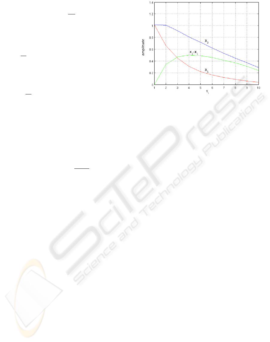
Figure 1: Effect of the modification of the time constant τ
1
on the state x
1
in the oscillatory neural network. τ
2
is kept
fixed(τ
2
= 1).
3.2 Feedback Design of the System
The torque amplitude of the oscillatory controller,
considering its frequency, may be too large for the
needs of the Roller Racer. Beside, the starting energy
for a vehicle is generally different from when it is
at full speed. So is the Roller Racer with the torque
control. It needs a transient oscillatory input which
might depend on friction biases and inertia. Thus we
create an angle feedback from the Roller Racer to the
oscillatory controller, which purpose is to constrain
the angle within some limits. We control the vehicle
in the forward direction which means the average
angle of the handlebar should be π (see (Jouffroy and
Jouffroy, 2006)).
To apply a correction to the torque generated, we
use the feedback to modify the time constants τ
i
of the
oscillatory controller’s output neurons. In Figure 1
we illustrate the effect on the amplitude of the output
neurons state when changing only one time constant
(τ
1
on the figure). As might be expected, the state of
each neuron output decreases. However the correc-
tion applies more to x
1
, and the amplitude difference
is maximum at τ ≈ 4. It is not really really desirable
to have one output which becomes zero as it prevents
the Roller Racer to get energy. Therefore we should
not have τ
i
being set too high.
We now define the transfer function, that con-
strains the angle within the boundaries [π − 1; π + 1]
and with a correction applied when τ
i
< 5, consid-
ering the effect on the amplitude reduced above this
limit. Note that the frequency is relatively not mod-
ified in this range (a frequency modification would
take place if all τ
i
where equally changed). The trans-
fer function g for the feedback is defined as
TORQUE CONTROL WITH RECURRENT NEURAL NETWORKS
111

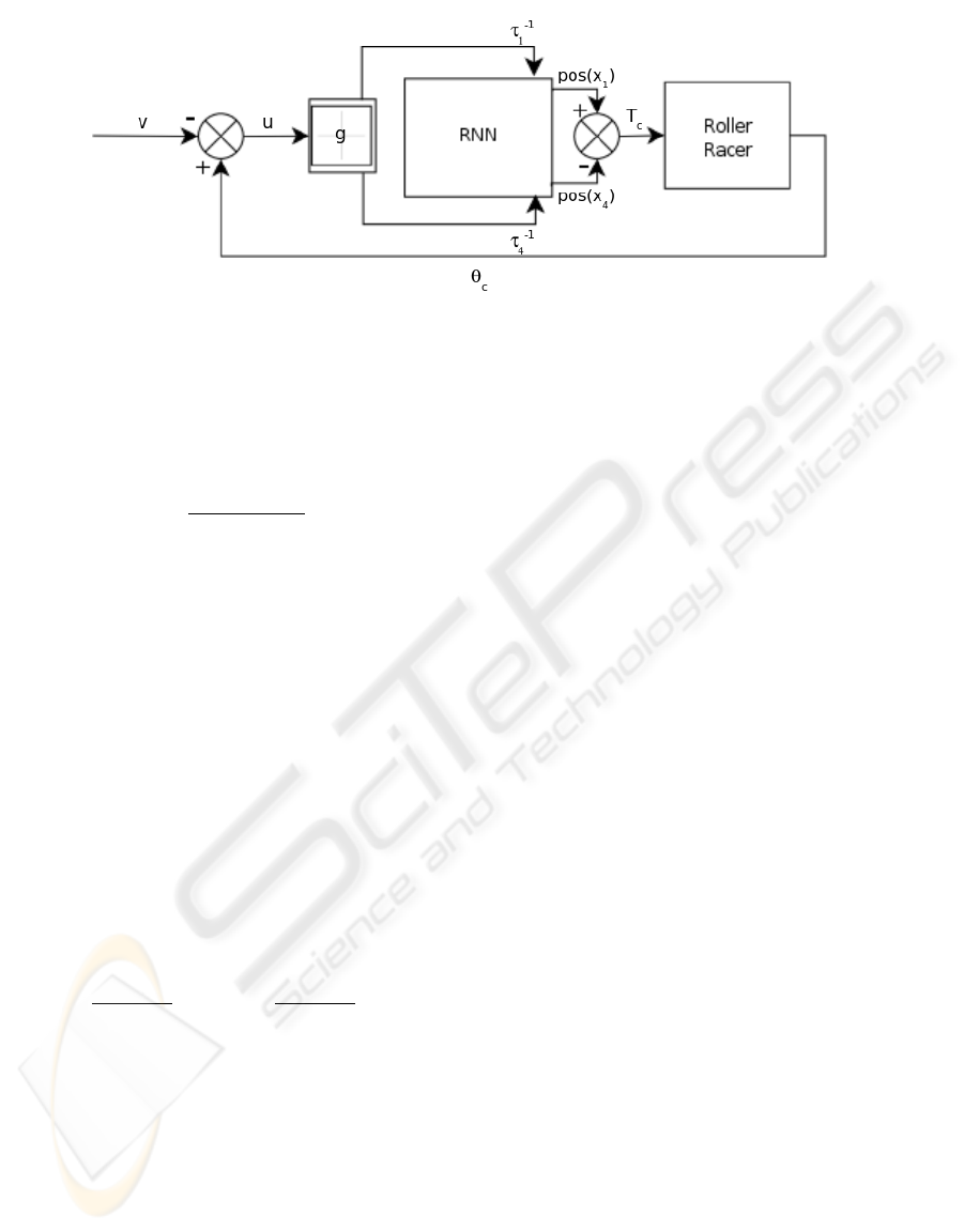
Figure 2: Control architecture of the Roller Racer. T
c
is the torque control applied to the vehicle. v is the angular input which
is obtained from the user direction control δ.
g(u) =

g
1
(u)
g
4
(u)

, (13)
with
g
1
(u) =
6
1 + e
−(6u−4.5)
, (14)
g
1
being the transfer function for the feedback to the
neuron 1, and g
4
(u) = −g
1
(u) to the neuron 4.
The formalization of these transfer functions has
been chosen so that they can be used as “feedback”
neurons, with the same neuron model as in (3) , re-
placing f
i
by g
i
.
The signal u ∈ R is the actual feedback signal which
is the difference between the angle of the handlebar
θ
c
(in radians) and the desired average angle control
v ∈ R. For the forward direction u is actually set as
u = θ
c
− v = θ
c
− (π + δ), (15)
where δ ∈ R is the user direction input, which is actu-
ally the continuous component control of the RNN.
The feedback information thus obtained is used to
modify the time constants τ
1
and τ
4
τ
−1
1
=
1
1 + g
1
(u)
and τ
−1
4
=
1
1 + g
4
(u)
(16)
The whole architecture is summarized in Figure 2.
3.3 Results
We present here the results of two different trials. In
both of them the purpose is to have a straight trajec-
tory along the x axis of a physical space reference.
The architecture is of course able to freely control the
vehicle in all directions but the simulations are not
shown.
In the first trial we start the RNN with a little energy
given to a neuron. The neuron 3 in the following sim-
ulation has the initial condition x
3
= 0.1.
In Figure 3 left, is plotted the angle of the han-
dlebar θ
c
which continuous component is π, for the
forward direction. It clearly shows the transient time
when the system is extracting itself from reaction
forces, until it reaches its permanent speed at around
40 timesteps. The transient period has an amplifying
oscillation around π because the RNN is also in its
transient state with little energy.
This transient activity of the RNN, is shown by the
very weak correction applied from the feedback g(u)
in Figure 3 right, and the low speed along the x axis in
Figure 3 bottom. One can clearly see on this graphics
of the right side of the figure, a little deviation during
this time. This is only the drawback of the transient
state of the RNN which does not provide a symmetric
gain, even if the angle is within the boundaries [π −
1;π + 1].
The correction applied once the vehicle is in its
permanent state shows that the RNN’s own oscillation
is not optimal and that a relearning could fix this. The
trajectory however becomes quite straight.
In the second trial we initialize the RNN with a
strong gain to see how the feedback behaves during
the transient period. We set x
3
= 1.
In Figure 4 left we can see that the amplitude
of the transient state of the RNN has been pushed
too high. The angle of the handlebar θ
c
does not
show anymore an amplifying oscillatory behavior,
and reach the boundaries we have specified. The cor-
rection from the feedback apply a high gain correction
(see Figure 4 right).
After t ≈ 40, as in the first trial, the symmet-
ric oscillations are recovered, and the correction re-
duces to the steady-state time in Figure 3 right. Inter-
estingly the correction has constrained the deviation
well, which is not higher than in the first trial, except
in the transient period. The vehicle also gets speed
earlier and the trajectory is also straight (Figure 4 bot-
tom).
ICINCO 2008 - International Conference on Informatics in Control, Automation and Robotics
112

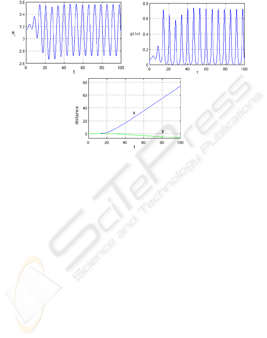
Figure 3: Simulation results when the RNN is initialized with a weak energy. Left: angle of the handlebar θ
c
. Right: feedback
correction g
1
(u). Bottom: trajectory evolution. During and after the transient times, little correction is applied.
4 CONCLUSIONS AND
DISCUSSION
Nature is a great source of inspiration for engi-
neers who deal with autonomous robots. Evolution
has found optimally-designed solutions for robustness
and adaptability in a changing environment, which are
exciting to discover. However, most of the research
in the control aspects of robots with neural networks
tackle the question of complex mechanics with many
degrees of freedom, and massive neural architectures,
which appear as “black boxes” designed by genetics
algorithms. This hides the dynamics of the neural
system and correlatively the opportunity to constitute
adaptive strategies.
In this work, we present a generalized version of the
teacher forcing learning algorithm, to build up an es-
timated oscillatory controller for a vehicle with one
degree of freedom, the Roller Racer. We create an
angular feedback such that the degree of freedom is
constrained within some boundaries. The purpose is
to prevent the vehicle to go out of control during its
transient state when it starts moving, as a consequence
of the oscillator being not adapted to this particular
moment.
Our simulation results show that the feedback
makes the vehicle to behave relatively well during
transient state, when the oscillator is initialized with a
weak energy or even a strong one. The deviation also
stays little. When the steady-state period is reached,
the vehicle moves in a straight line as expected.
From a design point of view, the correction
applied by the feedback system to the RNN, never
completely vanishes. This shows that a more optimal
oscillatory behavior can be obtained, though the
“default” one does not critically affect the system
with the help of a mutual entrainment between the
vehicle dynamics and the controller, as described first
by (Taga, 1994).
We are currently studying how an adaptive pro-
cess or observer, can modify permanently the RNN
when the average correction is too high. The outputs
of the network, with the help of the feedback, could be
the desired targets for a second network which could
thus be trained in parallel, with a partial teacher forc-
ing. However this is highly computationally expen-
sive, and not biologically viable.
The teacher forcing principle is made such that
an oscillatory behavior can be obtained with a gra-
dient descent algorithm. However, forcing the out-
puts of the network means disconnecting it, and thus
loosing the interesting desired target obtained with
feedback. Algorithms without direct gradient descent
evaluation techniques may be more appropriate (for
e.g. (Kailath, 1990)).
TORQUE CONTROL WITH RECURRENT NEURAL NETWORKS
113

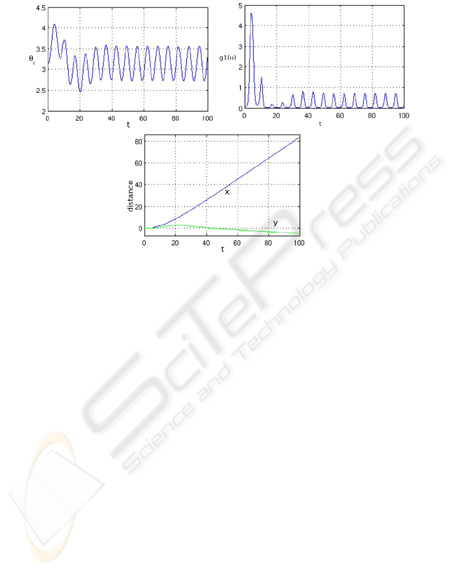
Figure 4: Simulation results when the RNN is initialized with a stronger energy. The correction is high during the transient
state. The deviation is not higher than in the first trial which shows the effective action of the feedback.
Beside, the constraint method we used in this arti-
cle can have some interest when studying the coupling
of oscillatory neural networks, for e.g. to synchronize
different joints. When we attach an oscillatory RNN
to another one which has a constraining feedback, we
can find coupling parameters which do not yield an
increase of the correction in the feedback. This con-
straint method thus helps to reduce the space to search
for suitable coupling parameters, and to better match
the desired phase relationship.
REFERENCES
Buono, P. and M.Golubitsky (2001). Models of central pat-
tern generators for quadruped locomotion. Journal of
Mathematical Biology, 42:291–326.
Ghigliazza, R. and P.Holmes (2004). A minimal model of
a central pattern generator and motoneurons for in-
sects locomotion. SIAM Journal on Applied Dynami-
cal Systems, 3(4):671–700.
Ijspeert, A. (2001). A connectionnist central pattern gener-
ator for the aquatic and terrestrial gaits of a simulated
salamander. Biological Cybernetics, 84:331–348.
Ishiguro, A., Otsu, K., Fujii, A., Uchikawa, Y., Aoki,
T., and Eggenberger, P. (2000). Evolving and adap-
tive controller for a legged-robot with dynamically-
rearranging neural networks. In Proceedings of
the Sixth International Conference on Simulation of
Adaptive Behavior, Cambridge, MA. MIT Press.
Jouffroy, G. and Jouffroy, J. (2006). A simple mechanical
system for studying adaptive oscillatory neural net-
works. IEEE International Conference on Systems,
Man and Cybernetics, pages 2584–2589.
Kailath, A. D. . T. (1990). Model-free distributed learning.
IEEE Trans. Neural Networks, 1(1):58–70.
Kamimura, A., Kurokawa, H., Yoshida, E., Tomita, K., Mu-
rata, S., and Kokaji, S. (2003). Automatic locomotion
pattern generation for modular robots. In Proceed-
ings of IEEE International Conference on Robotics
and Automation, pages 714–720.
Krishnaprasad, P. and Tsakriris, D. (1995). Oscilla-
tions, se(2)-snakes and motion control. New Orleans,
Louisiana.
Mori, T., Nakamura, Y., Sato, M., and Ishii, S. (2004). Rein-
forcement learning for cpg-driven biped robot. Nine-
teenth National Conference on Artifical Intelligence,
pages 623–630.
Taga, G. (1994). Emergence of bipedal locomotion through
entrainment among the neuro-musculo-skeletal sys-
tem and the environment. Physica D, 75:190–208.
Tsung, F. and Cottrell, G. (1993). Phase-space learning
for recurrent networks. Technical Report CS93-285,
Dept. Computer Science and Engineering, University
of California, San Diego.
Weiss, M. (1997). Learning oscillations using adaptive con-
trol. International Conference on artifical Neural Net-
works, pages 331–336.
ICINCO 2008 - International Conference on Informatics in Control, Automation and Robotics
114