EXPERIMENTAL OPEN-LOOP AND CLOSED-LOOP
IDENTIFICATION OF A MULTI-MASS
ELECTROMECHANICAL SERVO SYSTEM
Usama Abou-Zayed, Mahmoud Ashry and Tim Breikin
Control Systems Centre, The University of Manchester, PO BOX 88, M60 1QD, U.K.
Keywords: System identification, black-box model, recursive least square algorithm, local optimal controller, and
multi-mass servo systems.
Abstract: The procedure of system identification of multi-mass servo system using different methods is described in
this paper. Different black-box models are identified. Previous experimental results show that a model
consisting of three-masses connected by springs and dampers gives an acceptable description of the
dynamics of the servo system. However, this work shows that a lower order black-box model, identified
using off-line or on-line experiments, gives better fit. The purpose of this contribution is to present
experimental identification of a multi-mass servo system using different algorithms.
1 INTRODUCTION
An important step in designing a control system is
proper modeling of the system to be controlled. An
exact system model should produce output responses
similar to those of the actual system. The complexity
of most physical systems makes the development of
exact models infeasible. Therefore, in order to
design a controller that is reliable and easy to
understand in practice, simplified system models
should be obtained around operating points and\or
model order reduction (Ziaei, 2000).
System identification is an established modeling tool
in engineering and numerous successful applications
have been reported. The theory is well developed
(Ljung, 1999; Soderstrom, 1989), and there are
powerful software tools available, e.g., the System
Identification Toolbox (SIT) (Ljung, 1997).
Different physical models of electromechanical
servo systems based on multi-mass representation
were discussed in (Abou-Zayed, 2008). Using grey-
box off-line identification, inertial parameters and
parameters describing flexibilities were identified.
The physical parameters estimates showed no
variations in the mechanical parameters, and
acceptable variations in the electrical parameters.
Experimental results in (Abou-Zayed, 2008) show
that a model consisting of three masses connected by
springs and dampers gives an acceptable description
of the dynamics of the servo system. However, this
model is a six-order state-space model.
The objective of this paper is to present our recent
experimental studies on black-box open-loop and
closed-loop identification of a three-mass
electromechanical system. The closed-loop tests are
performed using a local-optimal controller.
The paper is organized as follows. In section 2,
the servo system is described briefly. In Section 3,
the results of black-box off-line identification are
presented. On-line open-loop and closed-loop
identification of the studied system is discussed in
section 4. Finally, Section 5 contains some
conclusions.
2 EXPERIMENTAL SETUP
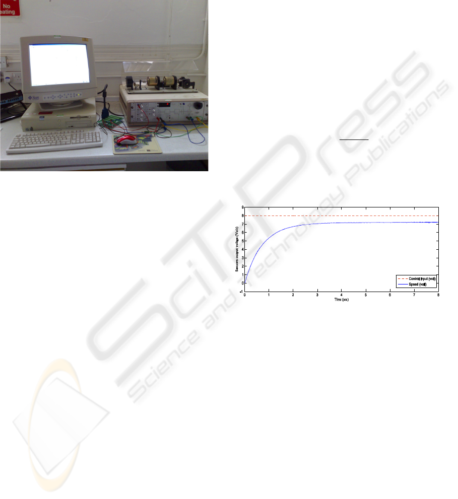
A view from the experimental setup is shown in
Fig.1. The DC servo mechanism setup to be studied
operates at ±10V input voltage with a permissible
output motor shaft speed of 2200 r.p.m. The shaft is
connected to an inertial load through a coupling gear
with ratio (r=1/30).The load shaft carries an absolute
position sensor with linear range ±10V. A personal
computer PC (Pentium III, 700 MHz, 256 MB
RAM), running the MATLAB software, is
188
Abou-Zayed U., Ashry M. and Breikin T. (2008).
EXPERIMENTAL OPEN-LOOP AND CLOSED-LOOP IDENTIFICATION OF A MULTI-MASS ELECTROMECHANICAL SERVO SYSTEM.
In Proceedings of the Fifth International Conference on Informatics in Control, Automation and Robotics - SPSMC, pages 188-193
DOI: 10.5220/0001502601880193
Copyright
c
 SciTePress

connected to the servo system setup through a data
acquisition card. This PC is used as a signal
generator for the servo system input. It also used as a
data logger to store the relevant system parameters
at fixed sample time. The third function is a digital
controller for closed-loop identification purposes.
Figure 1: Experimental setup.
The DC servo system setup, shown in Fig.1 can be
viewed as single input single output (SISO) for the
present case, where the motor armature voltage
a
v
is the input, while the output is the angular position
of the load
L
θ
. Since the measurement noise is
fairly small, a reasonable estimate of the load
angular speed
L
ω
is obtained for the identification
purpose. Therefore, the load angular speed will be
used as the output signal.
3 OFF-LINE IDENTIFICATION
OF SERVO SYSTEM
This section presents the results of the study and
realization of the off-line identification of servo
systems for different types of models with different
excitations. First, some dynamical properties of the
system are obtained using the process reaction curve
method. Then, black-box models, describing the
system, are identified.
3.1 Process Reaction Curve
Identification
It is one of the widely used approaches to
predetermine the dynamic behaviour of a system
before performing the data collection for system
identification. An input step signal change is applied
to the system, and the output response is measured.
Rise time, settling time, bandwidth, time constant,
time delay, and type of response can be determined
using the Process reaction curve (Ziegler, 1942).
System step response is shown in Fig.2. The sample
time chosen for this step test is 0.01sec to observe
the system dynamical behaviour. An 8V input
voltage (dashed line) is applied to the system. The
output response (solid line) acts like a first order
plus time delay system with average steady state
output 7.18V, rise time about 1.4sec, and bandwidth
around 1.6rad/s. Using the process reaction curve
method the system can be modeled as in the classical
case:
()
1
Ts
d
Ke
Gs
s
τ
−
=
+
(1)
where K is the steady state gain (K = 0.898), T
d
is
the time delay (T
d
= 10 ms), and τ is the time
constant (τ = 0.73sec).
Figure 2: Output response of a step input change.
3.2 Experiment Design
The results of the identification experiments
reported here are based on two data sets where the
excitation signal has different character:
Set 1: A sum of 16 sinusoids with amplitude 1.8 and
equidistant spacing in frequency, between 0.1 and
6.1 rad/sec. The resulting crest factor (Ljung, 1999)
is 1.8 due to the Schroeder phase choice (Schroeder,
1970). The time response and power spectrum of the
set are shown in Fig.3.
Set 2: A linear swept-frequency sinusoidal signal
with amplitude 9 and time-varying frequency over a
certain band ranges from 0.1 to 6.1rad/sec over a
certain time period 100sec. The resulting input
signal has a crest factor 1.42, and shown in Fig 4.
EXPERIMENTAL OPEN-LOOP AND CLOSED-LOOP IDENTIFICATION OF A MULTI-MASS
ELECTROMECHANICAL SERVO SYSTEM
189

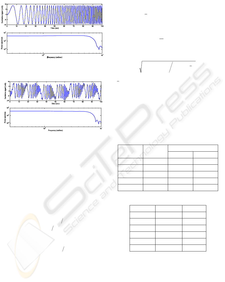
Figure 3: Multi-sine signal time response and power
spectrum.
Figure 4: Chirp sine signal time response and power
spectrum.
3.3 Black-box Transfer Function
Model Identification
The starting point is the general linear model
structure (Ljung, 1999),
,(,)()
y
(t)=G(q )u(t)+H q e t θθ (2)
where q denotes the shift operator.
Two different model structures will be studied, and
these are the ARX structure, defined by:
(, ) (,) (,),
(, ) 1 (,)
Gq Bq Aq
Hq Aq
θ
θθ
θθ
=
=
(3)
and the OE structure, where:
(, ) (,) (,),
(, ) 1
Gq Bq Fq
Hq
θ
θθ
θ
=
=
(4)
For the two model structures mentioned above, the
estimation of the model parameters will be carried
out generally using prediction error method (PEM).
The identification experiments are carried out using
the SIT (Ljung, 1997).
Tables 1, and 2 show the results of the estimated
models using data set1 for ARX and OE model
structures respectively. Both data sets show nearly
similar estimates. The notation (ModelStructure pzd)
denotes the p
th
order model with ‘z’ zeroes and
delay‘d’. The comparison is carried out using two
different quantities. The first is MSE as:
()
1
2
ˆ
() ()
1
N
M
SE y t y t
N
t
=−
∑
=
(5)
The second is the FIT:
() ()
()
()
()
22
ˆ
FIT 1 100%
11
NN
yt yt yt y
tt
⎛⎞
⎛⎞
⎜⎟
⎜⎟
=− − − ×
∑∑
⎜⎟
⎜⎟
⎜⎟
==
⎝⎠
⎝⎠
(6)
y is the mean value of the measured output.
Using k-step ahead predictors
ˆˆ
(| ;)yyttk
k
θ
=−
.The
two extreme predictors is defined as:
()()() () ()
11
ˆ
() 1
1
ytHqGqut Hqyt
−−
⎡⎤
=+−
⎢⎥
⎣⎦
(7)
()()
ˆ
()ytGqut=
∞
(8)
Table 1: Comparison of black-box ARX models.
fit
(
cross validation
)
%
Model MSE×10
-3
k
=1
k
=∞
ARX 211 5.95 96.01 85.80
ARX 311 2.29 97.72 80.25
ARX 411 0.76 98.44 84.28
ARX 511 0.58 98.76 83.00
ARX 611 0.35 99.03 82.50
Table 2: Comparison of black-box OE models.
Model MSE×10
-3
fit %
OE 211 39.90 85.53
OE 311 38.20 84.99
OE 321 38.30 84.98
OE 421 37.60 85.66
OE 611 37.70 85.72
OE 621 34.70 86.17
It is clear that for OE models, there is no difference
between both predictors. Otherwise, there is
considerable difference between them. The one-step
ahead predictor can give fits that “look good,” even
though the model may be bad. Therefore, the
simulation fit can be used for invalidating the bad
models.
ICINCO 2008 - International Conference on Informatics in Control, Automation and Robotics
190

4 ON-LINE IDENTIFICATION OF
SERVO SYSTEM
4.1 Open-loop System Identification
Experiments are performed to find the discrete-time
model that can best represent the system using RLS
method. Let the system model is given in the form:
11
()() ()(1)Az yt Bz ut
−−
=
− (9)
where z
-1
is the back shift operator, and
112
()1
12
112
()
12
n
a
Az az az a z
n
a
n
b
Bz b bz bz b z
on
b
−
−−−
=+ + + +
−
−−−
=+ + + +
""
""
(10)
A model of the system in (9) can be presented in the
form of
() ()
T
yt t
ϕ
θ =
(11)
where
θ is a vector of unknown parameters defined
by:
,,,,,
1
T
aab b
no n
ab
θ
⎡⎤
=
⎣⎦
"" ""
(12)
and φ is a vector of regression which consists of
measured values of inputs and outputs
( ) ( 1), , ( ), ( 1), , ( 1)
T
t yt yt n ut ut n
ab
ϕ
⎡⎤
=− − − − − − −
⎣⎦
"" "" (13)
The model given in (11) presents an accurate
description of the system. However, in this
expression the vector of system parameters
θ is
unknown. It is important to determine it by using
available data in signal samples at system output and
input. For that purpose a model of the system is
supposed
ˆ
ˆ
() () ( 1)
T
yt t t
ϕθ =− (14)
For the RLS algorithm to be able to update the
parameters at each sample time, it is necessary to
define an error. The model prediction error, ε(t) is a
key variable in RLS algorithm and is defined as
ˆ
ˆ
() () () () () ( 1)
T
tytytyt tt
εϕθ =−=− − (15)
The error ε(t) is the difference between the system
output and the estimated model output. This model
prediction error is used to update the parameter
estimates as
ˆˆ
() ( 1) () () ()tt Pttt
θθ ϕε =−+
(16)
where the estimator covariance matrix P(t) is
updated using
1
() () ( 1)
() ( 1)
() ( 1) ()
T
ttPt
Pt Pt I
p
T
tPt t
ϕϕ
λ
λϕ ϕ
⎡
⎤
−
⎢
⎥
=−−
⎢
⎥
+−
⎣
⎦
(17)
where the subscript ‘p’ is the dimension of the
identity matrix, p=n
a
+n
b
+1, λ is the forgetting
factor, 0<λ≤1. The property of the forgetting factor,
λ, is that λ controls the speed of parameter
convergence: λ=1 yields the slowest speed, but
provides the best robustness towards noise, and
decreasing values of λ result in increasing speed of
parameter convergence. In general, choosing
0.98<λ<0.995 gives a good balance between
convergence speed and noise susceptibility
(Alexander, 2001).
Application of RLS method demands supposition of
the initial values of P(t) and
ˆ
()t
θ . The technique
which is chosen as estimates and then allowed to
settle to their final values as the program goes
through several iterations. There is no unique way to
initialize the algorithm. One suggestion is using a
supposition that the system is an integrator of the
first order with unit gain to set
ˆ
(0)
θ
. While, a
standard choice of P(0) is the unit matrix scaled by a
positive scalar α, (i.e. P(0)=αI
p
), where α is
recommended to be chosen 1<α<10
3
depending on
the existence of prior knowledge about the system
parameters (Wellstead, 1991).
A square wave perturbation signal with a frequency
of approximately 0.2 of the system bandwidth
ensures that most of the square wave power,
associated with the first three harmonic components,
is inside the system bandwidth. A square wave
perturbation signal with a frequency of f=0.05Hz
that is superimposed on a step signal was applied to
the system input. The RLS algorithm is implemented
for experimental tests using SIMULINK and real-
time windows target.
Table 3: MSE for different estimated models.
Order 1
st
2
nd
3
rd
4
th
5
th
MSE 0.00617 0.00368 0.00357 0.00355 0.00392
For comparison purposes, Table 3 shows the MSE
calculated for different model orders. Third order
EXPERIMENTAL OPEN-LOOP AND CLOSED-LOOP IDENTIFICATION OF A MULTI-MASS
ELECTROMECHANICAL SERVO SYSTEM
191

model appears to be suitable for describing the
system. Further increase in the model order brought
no significant improvement.
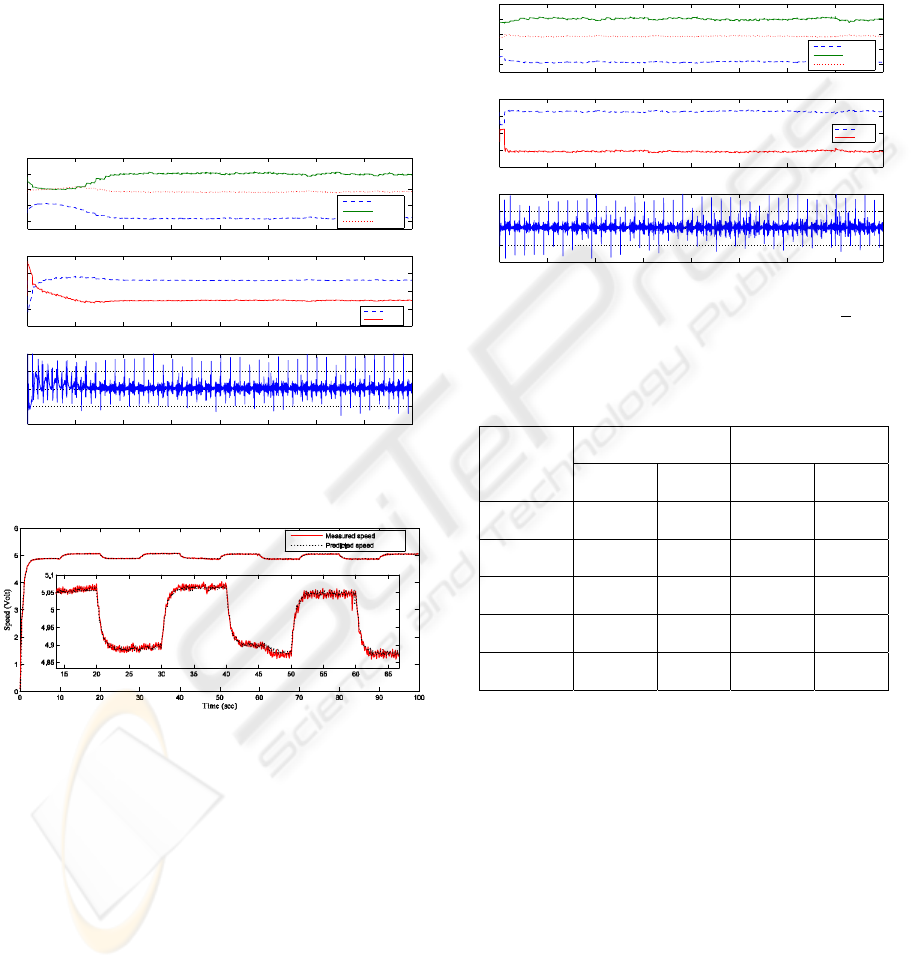
The performance of the estimated parameters and
the model output error for a third-order model are
shown in Fig. 5. Estimated parameters converge
after a certain time. The speed of parameter
convergence depends on the forgetting factor used.
Faster parameter convergence can be obtained if the
value of the forgetting factor is reduced, but noise
amplification. The measured system output and
predicted model output is shown in Fig. 6. It can be
seen that both output signals are in good agreement.
0 50 100 150 200 250 300 350 400
−0.2
−0.1
0
0.1
0.2
Time [Sec]
(c) Error signal
0 50 100 150 200 250 300 350 400
−2
−1
0
1
2
(a) Output parameters
0 50 100 150 200 250 300 350 400
−0.4
−0.2
0
0.2
0.4
(b) Input parameters
b1hat
b2hat
a1hat
a2hat
a3hat
Figure 5: Open-loop estimated parameters for 3rd order
model.
Figure 6: Measured and predicted speed for 3rd order
model.
4.2 Closed-loop System Identification
Closed-loop identification using direct method is
considered in this section. Knowledge of the
controller or the nature of the feedback is not a
certain requirement. A local-optimal controller
(Abou-Zayed, 2008) that provides stable closed-loop
servo operation is implemented, using SIMULINK
and real-time windows target.
The estimated parameters for the third-order model
are shown in Fig. 7. The parameters converge faster
than open-loop identification. Further, the variations
in the estimated parameters are smaller than that
obtained from the open-loop identification. This
phenomenon is due to the closed-loop feedback
control since the local-optimal controller filters high
frequency signal components and limits the
bandwidth.
0 50 100 150 200 250 300 350 40
0
−0.2
−0.1
0
0.1
0.2
Time [Sec]
(c) Error signal
0 50 100 150 200 250 300 350 40
0
−0.2
−0.1
0
0.1
0.2
(b) Input parameters
0 50 100 150 200 250 300 350 40
0
−2
−1
0
1
2
(a) Output parameters
b1hat
b2hat
a1hat
a2hat
a3hat
Figure 7: Closed-loop estimated parameters for 3
rd
order
model.
Table 4: Estimated parameters of third-order model for
open-loop and closed-loop experiments.
Open-loop Closed-loop
Parameters
Magnitude Variation Magnitude Variation
a
1
-1.821 0.204 -1.855 0.082
a
2
1.065 0.172 0.942 0.136
a
3
-0.122 0.144 -0.131 0.080
b
1
0.132 0.025 0.125 0.008
b
2
-0.105 0.029 -0.113 0.009
Table 4 shows the third-order parameters estimates
for both open-loop and closed-loop experiments. It
shows smaller variations for all parameters
estimated using closed-loop experiment. That comes
due to the closed-loop local-optimal control which
filters high frequency signal components and limits
the bandwidth
5 CONCLUSIONS
This paper presents theoretical and experimental
identification of a three-mass electromechanical
servo system using different algorithms. The aim of
ICINCO 2008 - International Conference on Informatics in Control, Automation and Robotics
192

this research is also to highlight some of the more
practical implications of plant identification and to
describe the well-established algorithm, recursive
least squares, used to perform system identification.
On-line open-loop and closed-loop identification of
the studied system is discussed. A real-time
implementation of the RLS estimator is presented
using SIMULINK and real-time windows target.
The application of the RLS method is also
demonstrated on a real-time experimental set-up
such that it is practical and easy to use. A third-order
discrete-time linear model is shown to be flexible
enough to fit the observations well. It also became
apparent that the order of the suitable linear model
was lower than the theoretical one. Closed-loop
identification gives faster parameters convergence
than open-loop identification. Further, the variations
in the estimated parameters are smaller than that
obtained from the open-loop identification. This
phenomenon is due to the closed-loop local-optimal
control which filters high frequency signal
components and limits the bandwidth.
ACKNOWLEDGEMENTS
The authors gratefully acknowledge the support of
this work by the EPSRC grant EP/C015185/1.
REFERENCES
Abou-Zayed, U., Ashry, M., & Breikin, T. (2008).
Implementation of local optimal controller based on
model identification of multi-mass electromechanical
servo system. Paper presented at the Proceedings of
the 27th IASTED International Conference on
Modelling, Identification, and Control.
Alexander, C. W., & Trahan, R. E. (2001). A comparison
of traditional and adaptive control strategies for
systems with time delay. ISA Transactions, 40(4),
353-368.
Ljung, L. (1997). System identification toolbox : for use
with MATLAB. Natick, Mass.: MathWorks Inc.
Ljung, L. (1999). System identification: theory for the
user. Upper Saddle River, N.J.; London: Prentice Hall
PTR: Prentice-Hall International.
Schroeder, M. (1970). Synthesis of low-peak factor signals
and binary sequences with low autocorrelation. IEEE
Trans. Inform. Theory, IT-16, 85-89.
Soderstrom, T. (1989). System identification. New York;
London: Prentice Hall.
Wellstead, P. E., & Zarrop, M. B. (1991). Self-tuning
systems: control and signal processing. Chichester:
Wiley.
Ziaei, K., & Sepehri, N. (2000). Modeling and
identification of electrohydraulic servos.
Mechatronics, 10(7), 761-772.
Ziegler, J. G., & Nichols, N. B. (1942). Optimum settings
for automatic controllers. Transactions of the ASME,
64, 759-768.
EXPERIMENTAL OPEN-LOOP AND CLOSED-LOOP IDENTIFICATION OF A MULTI-MASS
ELECTROMECHANICAL SERVO SYSTEM
193