NONLINEAR SYSTEM IDENTIFICATION USING
DISCRETE-TIME NEURAL NETWORKS WITH
STABLE LEARNING ALGORITHM
Talel Korkobi, Mohamed Djemel
Institute of Problem Solving, XYZ University, Intelligent Control, design & Optimization of complex Systems
National Engineering School of Sfax - ENIS, B.P. W, 3038 Sfax, Tunisia
Mohamed Chtourou
Intelligent Control, design & Optimization of complex Systems
National Engineering School of Sfax - ENIS, B.P. W, 3038 Sfax, Tunisia
Keywords: Stability, neural networks, identification, backpropagation algorithm, constrained learning rate, Lyapunov
approach.
Abstract: This paper presents a stable neural sytem identification for nonlinear systems. An input output discrete time
representation is considered. No a priori knowledge about the nonlinearities of the system is assumed. The
proposed learning rule is the backpropagation algorithm under the condition that the learning rate belongs
to a specified range defining the stability domain. Satisfying such condition, unstable phenomenon during
the learning process is avoided. A Lyapunov analysis is made in order to extract the new updating
formulation which contain a set of inequality constraints. In the constrained learning rate algorithm, the
learning rate is updated at each iteration by an equation derived using the stability conditions. As a case
study, identification of two discrete time systems is considered to demonstrate the effectiveness of the
proposed algorithm. Simulation results concerning the considered systems are presented.
1 INTRODUCTION
The area of system identification has received
significant attention over the past decades and now it
is a fairly mature field with many powerful methods
available at the disposal of control engineers. Online
system identification methods to date are based on
recursive methods such as least squares, for most
systems that are expressed as linear in the
parameters (LIP).
To overcome this LIP assumption, neural networks
(NNs) are now employed for system identification
since these networks learn complex mappings from a
set of examples. Due to NN approximation
properties as well as the inherent adaptation features
of these networks, NN present a potentially
appealing alternative to modeling of nonlinear
systems.
Moreover, from a practical perspective, the massive
parallelism and fast adaptability of NN
implementations provide additional incentives for
further investigation.
Several approaches have been presented for system
identification without using NN and using NN
(Narendra and Parthasarathy, 1990) (Boskovic and
Narendra 1995). Most of the developments are done
in continuous time due to the simplicity of deriving
adaptation schemes. To the contrary, very few
results are available for the system identification in
discrete time using NNs. However, most of the
schemes for system identification using NN have
been demonstrated through empirical studies, or
convergence of the output error is shown under ideal
conditions (Ching-Hang Lee and al, 2002).
Others (Sadegh, 1993) have shown the stability of
the overall system or convergence of the output error
using linearity in the parameters assumption. Both
recurrent and dynamic NN, in which the NN has its
own dynamics, have been used for system
identification.
351
Korkobi T., Djemel M. and Chtourou M. (2008).
NONLINEAR SYSTEM IDENTIFICATION USING DISCRETE-TIME NEURAL NETWORKS WITH STABLE LEARNING ALGORITHM.
In Proceedings of the Fifth International Conference on Informatics in Control, Automation and Robotics - ICSO, pages 351-356
DOI: 10.5220/0001504403510356
Copyright
c
 SciTePress

Most identification schemes using either multilayer
feedforward or recurrent NN include identifier
structures which do not guarantee the boundedness
of the identification error of the system under
nonideal conditions even in the open-loop
configuration.
Recent results show that neural network technique
seems to be very effective to identify a broad
category of complex nonlinear systems when
complete model information cannot be obtained.
Lyapunov approach can be used directly to obtain
stable training algorithms for continuous-time neural
networks (Ge, Hang, Lee, Zhang, 2001),
(Kosmatopoulos, Polycarpou, Christodoulou,
Ioannou, 1995) (Yu, Poznyak, Li, 2001). The
stability of neural networks can be found in (Feng,
Michel, 1999)and (Suykens, Vandewalle, De Moor,
1997). The stability of learning algorithms was
discussed in (Jin, Gupta, 1999) and (Polycarpou,
Ioannou 1992).
It is well known that normal identification
algorithms are stable for ideal plants (Ioannou, Sun,
2004). In the presence of disturbances or unmodeled
dynamics, these adaptive procedures can go to
instability easily. The lack of robustness in
parameters identification was demonstrated in (E.
Barn, 1992) and became a hot issue in 1980s.
Several robust modification techniques were
proposed in (Ioannou, Sun, 2004). The weight
adjusting algorithms of neural networks is a type of
parameters identification, the normal gradient
algorithm is stable when neural network model can
match the nonlinear plant exactly (Polycarpou,
Ioannou 1992). Generally, some modifications to the
normal gradient algorithm or backpropagation
should be applied, such that the learning process is
stable. For example, in (L. Jin, M.M. Gupta, 1999)
some hard restrictions were added in the learning
law, in (Polycarpou, Ioannou 1992) the dynamic
backpropagation was modified with stability
constraints.
The paper is organized as follows. Section II
describes the adopted identification scheme. In
section III and through a stability analysis a
constrained learning rate algorithm is proposed to
provide stable adaptive updating process. two simple
simulation examples give the effectiveness of the
suggested algorithm in section VI.
2 PRELIMINARIES
The main concern of this section is to introduce the
feedfarward neural network adopted architechture
and some concepts of backpropagation training
algorithm. Consider the following discrete-time
input-output nonlinear system
[
]
)1()......(),1().......()1( +−
+
−
=
+
mkukunkykyfky
(1)
The neural model for the plant can be expressed as
[
]
VWkYFky ,),()1(
ˆ
=
+
(2)
Where
)(),1(),....1(),(()( kunkykykykY +−
−
=
))1(......,),........1(, +−
−
mkuku
and W and V is the weight parameter vector for the
neural model.
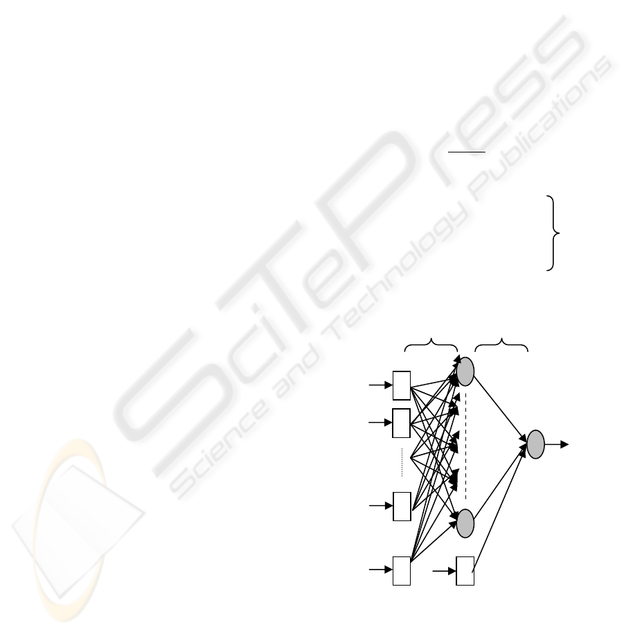
A typical multilayer feedfarward neural network is
shown in Figure 1, where I
i
is the ith neuron input,
Oj is the jth neuron output i, j and k indicate
neurons, wij is the weight between neuron i and
neuron j. For the ith neuron, the nonlinear active
function is defined as
x
e
xf
−
+
=
1
1
)(
(3)
The output y
m
(k) of the considered NN is
∑
++
=
=
1
1
mn
i
ijij
wxI
; O
j
= f (I
j
) ; j=1,….,m
(4)
∑
=
=
N
j
jj
VOI
1
'
; y
m
(k) = f (I’) ; k=1,...,N
Figure 1: Feedforward neural model.
Training the neural model consists on the adjustment
the weight parameters so that the neural model
emulates the nonlinear plant dynamics. Input–output
examples are obtained from the operation history of
the plant.
y
m
x
2
x
1
x
1
Wi
j
V
j
1
1 1
ICINCO 2008 - International Conference on Informatics in Control, Automation and Robotics
352

Using the gradient decent, the weight connecting
neuron i to neuron j is updated as
)(
)(
)()1(
kW
kJ
kWkW
ij
ijij
∂
∂
⋅−=+
ε
)(
)(
)()1(
kV
kJ
kVkV
j
jj
∂
∂
⋅−=+
ε
(5)
Where
[]
2
)1()1(
2
1
)( +−+= kykykJ
m
ε is the learning rate. The partial derivatives are
calculated with respect to the vector of weights W.
() j
m
j
j
OkykyIf
kV
kJ
))1()1(('
)(
)(
+−+⋅=
∂
∂
() ()
ij
m
L
j
jj
ij
xVkykyIfIf
kw
kJ
⎥
⎦
⎤
⎢
⎣
⎡
+−+=
∂
∂
∑
=
))1()1((''
)(
)(
1
(6)
Backpropagation algorithm has become the most
popular one for training of the multilayer perceptron
. Generally, some modifications to the normal
gradient algorithm or backpropagation should be
applied, such that the learning process is stable. For
example, in (
B. Egardt, 1979) some hard restrictions
were added in the learning law, in (
J.A.K. Suykens, J.
Vandewalle, B. De Moor, 1997) the dynamic
backpropagation was modified with stability
constraints
.
3 STABILITY ANALYSIS
In the literature, the Lyapunov synthesis (Z.P. Jiang,
Y. Wang, 2001), (W. Yu, X. Li, 2001) consists on the
selection of a positive function candidate V which
lead to the computation of an adaptation law
ensuring it’s decrescence
, i.e 0≤V
&
for continuous
systems and
0)()1()(
≤
−+=Δ kVkVkV for
discrete time systems. Under these assumptions the
function V is called Lyapunov function and garantee
the stability of the system. Our objective is the
determination of a stabilizing adaptation law
ensuring the stability of the identification scheme
presented below and the boundness of the output
signals. The following assumptions are made for
system (1)
Assumption 1. The unknown nonlinear function f(·)
is continuous and differentiable.
Assumption 2.
System output y(k) can be measured
and its initial values are assumed to remain in a
compact set
Ω
0
.
3.1 Theorem
The stability of the identification scheme is
guaranteed for a learning rate verifying the
following inequality :
∑∑
⎟
⎟
⎠
⎞
⎜
⎜
⎝
⎛
∂
∂
+
⎟
⎟
⎠
⎞
⎜
⎜
⎝
⎛
∂
∂
⎥
⎦
⎤
⎢
⎣
⎡
⎟
⎟
⎠
⎞
⎜
⎜
⎝
⎛
∂
∂
+
∂
∂
≤≤
ij
j
ji
ij
TT
kV
J
kW
J
kV
kV
J
kW
kW
J
tr
2
,
2
)()(
)(
)(
)(
)(
2
0
ε
(7)
Where W, V are respectivly the vector weight
between the inputs and the hidden layer and the
vector weight between the hidden layer and the
outputs layer. i denote the ith input and j the jth
hidden neuron.
3.2 Proof
Considering the Lyapunov function:
(
)
)(
~
)(
~
)(
~
)(
~
)( kVkVkWkWtrkV
TT
L
+=
(8)
Where
tr(.) denotes the matrix trace operation.
*
*
)()(
~
)()(
~
WkWkW
VkVkV
−=
−=
*
W
denotes the optimal vector weight between the
inputs and the hidden layer .
*
V
denotes the optimal vector weight between the
hidden layer and the outputs.
The computation of the
)(kV
L
Δ
expression leads to :
(
)
[
]
)1(
~
)1(
~
)1(
~
)1(
~
)()1()( +++++=−+=Δ kVk
T
VkWk
T
WtrkVkVk
L
V
(
)
[
]
)(
~
)(
~
)(
~
)(
~
kVkVkWkWtr
TT
+−
(9)
The adopted adaptation law is the gradient
algorithm. We have:
*
)(
)()1(
~
W
kW
J
kWkW −
∂
∂
−=+ ε
*
)(
)()1(
~
V
kV
J
kVkV −
∂
∂
−=+ ε
Where the partial derivatives are expressed as
)(
)1(
)1()( kW
ky
ky
J
kW
J
∂
+
∂
+∂
∂
=
∂
∂
(10)
)(
)1(
)1()( kV
ky
ky
J
kV
J
∂
+
∂
+∂
∂
=
∂
∂
Our field of interest covers the black box systems.
The partial derivatives denoting the system dynamic
are approximated as follow:
NONLINEAR SYSTEM IDENTIFICATION USING DISCRETE-TIME NEURAL NETWORKS WITH STABLE
LEARNING ALGORITHM
353

)(
)1(
)(
)1(
kW
ky
kW
ky
m
∂
+∂
≈
∂
+∂
(11)
)(
)1(
)(
)1(
kV
ky
kV
ky
m
∂
+∂
≈
∂
+∂
The approximated partial derivatives are given
through:
i
N
j
jj
mm
ij
xOOjVkekyky
kW
J
⎥
⎦
⎤
⎢
⎣
⎡
−+−+=
⎥
⎥
⎦
⎤
⎢
⎢
⎣
⎡
∂
∂
∑
=1
)1.().1,().()).1(1)(1(
)(
[]
j
mm
j
Okekyky
kV
J
).()).1(1)(1(
)(
+−+=
⎥
⎦
⎤
⎢
⎣
⎡
∂
∂
(12)
Adopting the variables A and B defined by:
(
)
(
)
)(
~
)(
~
)1(
~
)1(
~
kWkWtrkWkWtrA
TT
−++=
)(
~
)(
~
)1(
~
)1(
~
kVkVkVkVB
TT
−++=
The )(kVΔ expression i s calculated as :
BAkV +=Δ )(
⎟
⎟
⎠
⎞
⎜
⎜
⎝
⎛
∂
∂
−
⎥
⎦
⎤
⎢
⎣
⎡
∂
∂
∂
∂
= )(
~
)(
2
)()(
2
kW
kW
J
kW
J
kW
J
tr
T
εε
⎟
⎟
⎠
⎞
⎜
⎜
⎝
⎛
∂
∂
−
⎥
⎦
⎤
⎢
⎣
⎡
∂
∂
∂
∂
+ )(
~
)(
2
)()(
2
kV
kV
J
kV
J
kV
J
T
εε
⎟
⎟
⎠
⎞
⎜
⎜
⎝
⎛
⎟
⎠
⎞
⎜
⎝
⎛
∂
∂
−
⎥
⎦
⎤
⎢
⎣
⎡
∂
∂
=
∑
)(
~
)(
2
)(
,
2
2
kW
kW
J
tr
kW
J
T
jiij
εε
⎟
⎟
⎠
⎞
⎜
⎜
⎝
⎛
∂
∂
−
⎥
⎦
⎤
⎢
⎣
⎡
∂
∂
+
∑
)(
~
)(
2
)(
2
2
kV
kV
J
kV
J
T
j
j
εε
⎟
⎟
⎠
⎞
⎜
⎜
⎝
⎛
⎥
⎦
⎤
⎢
⎣
⎡
∂
∂
+
⎥
⎦
⎤
⎢
⎣
⎡
∂
∂
=
∑∑
j
j
ji
ij
kV
J
kW
J
2
,
2
2
)()(
ε
⎟
⎠
⎞
⎜
⎝
⎛
⎟
⎠
⎞
⎜
⎝
⎛
∂
∂
+
∂
∂
− )(
~
)(
)(
~
)(
2 kW
kW
J
trkV
kV
J
TT
ε
⎟
⎟
⎠
⎞
⎜
⎜
⎝
⎛
⎥
⎦
⎤
⎢
⎣
⎡
∂
∂
+
⎥
⎦
⎤
⎢
⎣
⎡
∂
∂
≤
∑∑
j
j
ji
ij
kV
J
kW
J
2
,
2
2
)()(
ε
⎟
⎠
⎞
⎜
⎝
⎛
⎟
⎠
⎞
⎜
⎝
⎛
∂
∂
+
∂
∂
− )(
)(
)(
)(
2 kW
kW
J
trkV
kV
J
TT
ε
ε
β
ε
α
⋅⋅−⋅≤ 2
2
Where
∑∑
⎥
⎦
⎤
⎢
⎣
⎡
∂
∂
+
⎥
⎦
⎤
⎢
⎣
⎡
∂
∂
=
jjjiij
kV
J
kW
J
2
,
2
)()(
α
⎟
⎠
⎞
⎜
⎝
⎛
∂
∂
+
∂
∂
= )(
)(
)(
)(
kW
kW
J
trkV
kV
J
TT
β
The stability condition
0)( ≤
Δ
kV
is satisfied only
if :
02
2
≤
⋅
⋅
−
⋅
ε
β
ε
α
(13)
Solving this ε second degree equation lead to the
establishment of the condition (7) :
0)(
≤
Δ
kV
if ε satisfies the following condition :
s
ε
ε
≤
≤
0
where
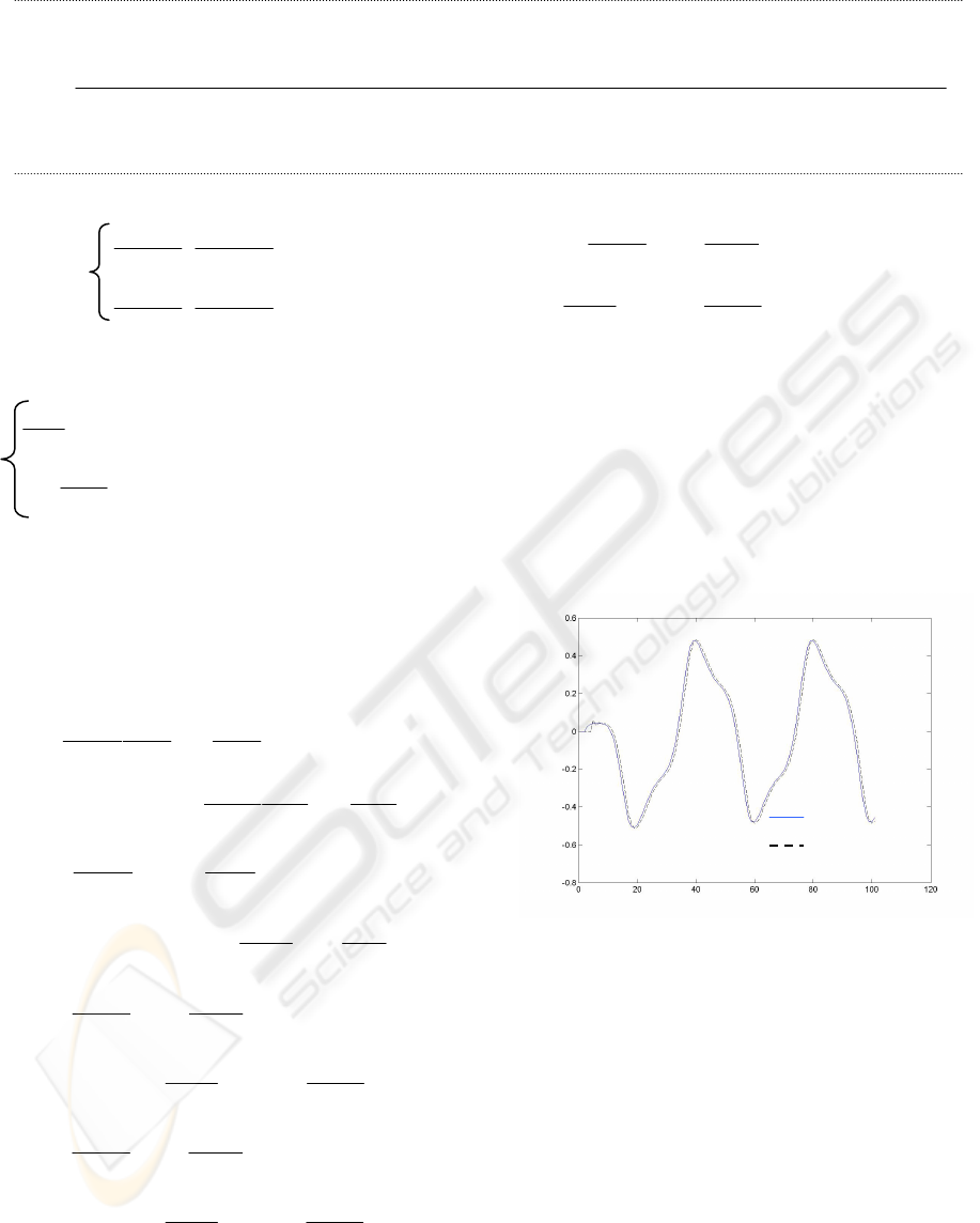
Figure 2: Evolution of the system output and the neural
model output (
domainstability
∈
ε
).
4 SIMULATION RESULTS
In this section two discrete time systems are
considered to demonstrate the effectivness of the
result discussed below.
4.1 First Order System
The considered system is a famous one in the
litterature of adaptive neural control and
identification. The discrete input-output equation is
defined by:
System
Neural model
[]
[]
[] {}
[]
[] ()
∑∑∑
∑
+−++
⎟
⎟
⎠
⎞
⎜
⎜
⎝
⎛
⎥
⎦
⎤
⎢
⎣
⎡
−+−+
⎢
⎢
⎣
⎡
⎜
⎜
⎝
⎛
⋅+−++⋅
⎭
⎬
⎫
⎩
⎨
⎧
⎥
⎦
⎤
⎢
⎣
⎡
−+−+
=
=
∈
∈
∈
=
j
j
mm
ji
i
N
j
jj
j
mm
T
mj
j
mm
T
ni
mj
i
N
j
jj
j
mm
s
OkekykyxOOVkekyky
VOkekykykWxOOVkekykytr
2
,
2
1
1
1
1
1
1
1
).()).1(1)(1()1.(.).()).1(1)(1(
).()).1(1)(1()()1.(.).()).1(1)(1(2
L
L
L
ε
ICINCO 2008 - International Conference on Informatics in Control, Automation and Robotics
354

3
2
)(
)(1
)(
)1( ku
ky
ky
ky +
+
=+
(15)
For the neural model , a three-layer NN was
selected with two inputs, three hidden and one
output nodes. Sigmoidal activation functions were
employed in all the nodes.
The weights are initialized to small random values.
The learning rate is evaluated at each iteration
through (14). It is also recognized that the training
performs very well when the learning rate is small.
As input signal, a sinusoidal one is chosen which
the expresion is defined by:
(
)
5
05.0cos5.0)(
π
π +⋅= kku
(16)
The simulations are realized in the two cases
during 120 iterations. Two learnning rates values
are fixed in and out of the learning rate range
presented in (7).Simulation results are given
through the following figures :
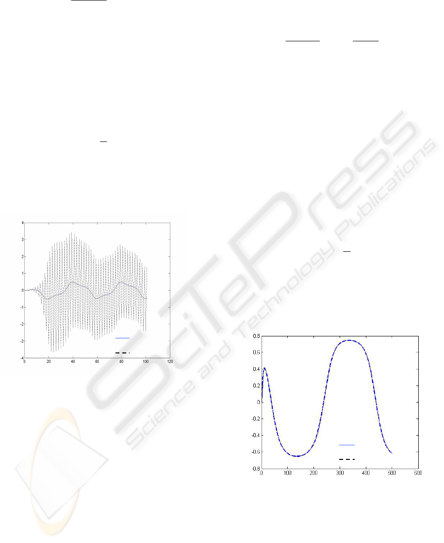
Figure 3 : Evolution of the system output and the neural
model output (
domainstability∉
ε
).
4.1.1 Comments
Fig 2 and Fig 3 show that if the learning rate
belongs to the range defined in (7), the stability of
the identification scheme is garanteed. It is shown
through this simulation that the identification
objectives are satisfied. Out this variation domain
of the learning rate, the identification is instable
and the identification objectives are unreachable.
4.2 Second Order System
The second example concerns a discrete time
system given by:
[
] )1(5,0)1(tanh50y(k) −+−= kuk ϕ
where
(
)
⎟
⎟
⎠
⎞
⎜
⎜
⎝
⎛
−
+
−−
+
= )1(
)(1
)(
8)1(
3
)(24
2.10(k)
2
2
2
ky
ku
ku
ky
ky
ϕ
(17)
The process dynamic is interesting. In fact it has
the behaviour of a first order law pass filter for
inputs signal amplitude about 0.1, the behaviour of
a linear second order system in the case of small
amplitudes (0,1 < |u| < 0,5) and the behaviour of a
non linear second order system in the case of great
inputs amplitudes (0,5 < |u| < 5) (
Ching-Hang Lee
and al, 2002).
For the neural model , a three-layer NN was
selected with three inputs, three hidden and one
output nodes. Sigmoidal activation functions were
employed in all the nodes.
The weights are initialized to small random values.
The learning rate parameter is computed
instantaneously. As input signal, a sinusoidal one
is chosen which the expresion is defined by:
(
)
3
005.0cos5.0)(
π
π +⋅= kku
(18)
The simulations are realized in the two cases. Two
learnning rates values are fixed in and out of the
learning rate range presented in (7).
Simulation results are given through the following
figures:
Figure 4: Evolution of the system output and the neural
model output (
domainstability
∈
ε
).
System
Neural model
System
Neural model
NONLINEAR SYSTEM IDENTIFICATION USING DISCRETE-TIME NEURAL NETWORKS WITH STABLE
LEARNING ALGORITHM
355

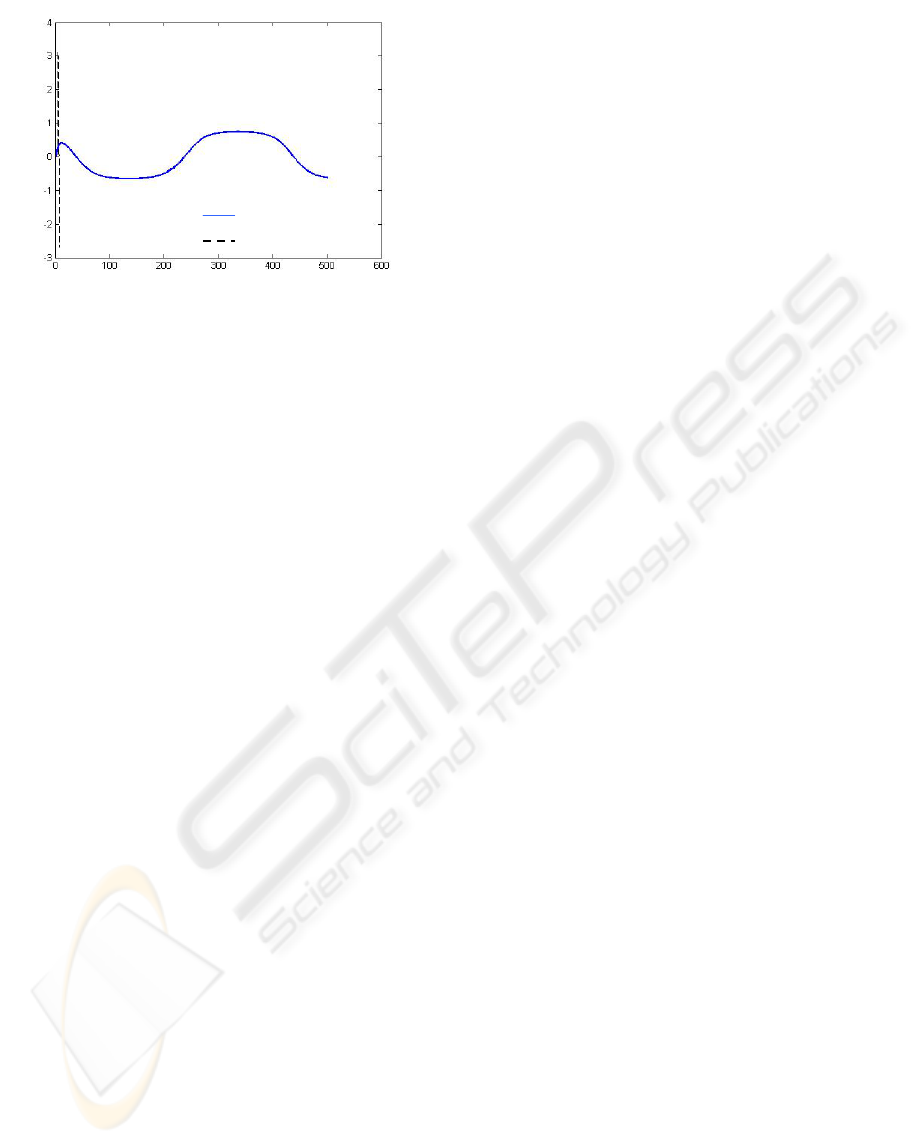
Figure 5: Evolution of the system output and the neural
model output (
domainstability∉
ε
).
4.2.1 Comments
Here we made a comparative study between an
arbitrary choice of a learning rate out side of the
stability domain and a constrained choice verifying
the stability condition and guarantying tracking
capability. The simulation results schow that a
learning rate in the stability domain ensure the
stability of the identification scheme.
5 CONCLUSIONS
To avoid unstable phenomenon during the learning
process, constrained learning rate algorithm is
proposed. A stable adaptive updating processes is
guaranteed. A Lyapunov analysis is made in order
to extract the new updating formulations which
under inequality constraint. In the constrained
learning rate algorithm, the learning rate is updated
at each iterative instant by an equation derived
using the stability conditions. The applicability of
the approach presented is illustrated through two
simulation examples.
REFERENCES
B. Egardt, 1979. Stability of adaptive controllers. in:
Lecture Notes in Control and Information Sciences
20, Springer-Verlag, Berlin.
Z. Feng, A.N. Michel, 1999. Robustness analysis of a
class of discrete-time systems with applications to
neural networks, in: Proceedings of American
Control Conference, San Deigo, pp. 3479–3483.
S.S. Ge, C.C. Hang, T.H. Lee, T. Zhang, 2001: Stable
Adaptive Neural Network Control, Kluwer
Academic, Boston.
P. A. Ioannou, J. Sun, 2004. Robust Adaptive Control,
Information Sciences 158, 31–147, Prentice-Hall,
Upper Saddle River.
L. Jin, M.M. Gupta, 1999. Stable dynamic
backpropagation learning in recurrent neural
networks, IEEE Trans. Neural Networks 10 (6) ,
1321–1334.
Z. P. Jiang, Y. Wang, 2001. Input-to-state stability for
discrete-time nonlinear systems, Automatica 37 (2) ,
857–869.
E. B. Kosmatopoulos, M.M. Polycarpou, M.A.
Christodoulou, P.A. Ioannou, 1995. High-order
neural network structures for identification of
dynamical systems, IEEE Trans. Neural Networks 6
(2), 431–442.
M. M. Polycarpou, P.A. Ioannou 1992. Learning and
convergence analysis of neural-type structured
networks, IEEE Trans. Neural Networks 3 (1) ,39–
50.
J. A. K. Suykens, J. Vandewalle, B. De Moor, 1997.
NLq theory: checking and imposing stability of
recurrent neural networks for nonlinear modelling,
IEEE Trans. Signal Process (special issue on neural
networks for signal processing) 45 (11) , 2682–2691.
W. Yu, X. Li, 2001. Some stability properties of
dynamic neural networks, IEEE Trans. Circuits
Syst., Part I 48 (1) , 256–259.
W. Yu, A.S. Poznyak, X. Li, 2001. Multilayer dynamic
neural networks for nonlinear system on-line
identification, Int. J. Control 74 (18), 1858–1864.
E. Barn, 1992. Optimisation for training neural nets,
IEEE Trans. Neural Networks 3 (2) , 232–240.
Ching-Hang Lee and al, 2002. Control of Nonlinear
Dynamic Systems Via adaptive PID Control Scheme
with Daturation Bound, International Journal of
Fuzzy Systems, Vol. 4 No. 4 ,922-927.
K. S. Narendra and K. Parthasarathy, 1990.
Identification and control of dynamical systems
using neural networks, IEEE Transaction Neural
Networks, vol.1, pp.4–27, Mar.
J. D. Boskovic and K.S.Narendra 1995. Comparison of
linear nonlinear and neural-network based adaptive
controllers for a class of fed-batch fermentation
process, Automatica, vol. 31, no. 6, pp. 537-547.
System
Neural model
ICINCO 2008 - International Conference on Informatics in Control, Automation and Robotics
356