
ZISC Neuro-Computer for Task Complexity Estimation
in T-DTS Framework
Ivan Budnyk, Abdennasser Chebira and Kurosh Madani
Images, Signals and Intelligent Systems Laboratory (LISSI/EA 3956), University Paris 12
Senart-Fontainebleau Institute of Technology, Bat A, Av. Pierre Point, 77127 Lieusaint, France
Abstract. This paper deals with T-DTS, a self-organizing information process-
ing system and especially with its complexity estimation mechanism which is
based on a ZISC © IBM ® neuro-computer. The above-mentioned mechanism
has been compared with a number probabilistic complexity estimation tech-
niques already implemented in T-DTS.
1 Introduction
This work connects closely the Tree-like Divide to Simplify (T-DTS) [1] framework,
which is a hybrid multiple Neural Networks software platform constructing a decom-
posed-tree of neural structures aiming to solve complex classification problems using
“divide and conquer” paradigm. In other words, the solution of a complex classifica-
tion task is approached by dividing the initial complex task into a set of classification
sub-problems with reduced complexity. So, the splitting mechanism and associated
policy play a key role in tree-like self-organization to obtain multi-neural structure as
well as in its classification performances. In T-DTS, the splitting is performed using a
complexity estimation mechanism acting as a regulation loop on decomposition proc-
ess [2]. If several probabilistic (or statistical) complexity estimation perspectives have
been investigated in [3], an appealing slant consists of using Artificial Neural Net-
work’s (ANN) learning issued mechanisms as indicators for complexity estimation:
especially, those modifying the ANN topology. Among various available ANNs, a
promising candidate is the Restricted Coulomb Energy (RCE) neural model and the
relatively simple learning mechanism of such ANN, modifying directly its topology
(number of neurons in hidden layer). Moreover, the standard CMOS based ZISC ©
IBM ® neuro-computer, implementing this kind of neural model, is an attractive
feature offering hardware implementation potentiality of a ZISC based diffi-
culty/complexity tasks estimator [4]. If the expected impact of the complex task de-
composition is to increase the classification quality, an additional impact of a ZISC
based difficulty/complexity tasks estimator is the decreasing of learning time (gener-
ally, processing time consumer).
In this paper we compare the ZISC based complexity estimation indicator with
those based on probabilistic (or statistical) measures described in [2] and [3], already
Budnyk I., Chebira A. and Madani K. (2008).
ZISC Neuro-Computer for Task Complexity Estimation in T-DTS Framework.
In Proceedings of the 4th International Workshop on Artificial Neural Networks and Intelligent Information Processing, pages 18-27
DOI: 10.5220/0001509200180027
Copyright
c
SciTePress

implanted in T-DTS. We compare obtained results in order to show special niche
which takes ZISC complexity estimator among the others.
In Section 2 we describe T-DTS concept and its software platform, highlighting key
role of complexity estimating unit and providing its’ component analysis. Section 3
presents ZISC based complexity estimating issue and its influence on T-DTS per-
formance. Section 4 gives results of the above-mentioned comparison obtained on the
basis of a simple 2D benchmark and two real-world classification problems (available
in UCI Machine Learning depository). Section 5 includes summary and our further
progress.
2 Hybrid Multiple Neural Networks Framework - T-DTS
In essence, T-DTS is a modular structure [5]. The purpose is based on the use of a set
of specialized mapping Neural Network, called Processing Units (PU), supervised by
a set of Decomposition Units (DU). Decomposition Units are a prototypes based on
Neural Networks. Processing Units are modeling algorithms of Artificial Neural Net-
works origin. Thus, T-DTS paradigm allows us to build a tree structure of models in
the following way:
• at the nodes level(s) - the input space is decomposed into a set of optimal
sub-spaces of the smaller size;
• at the leaves level(s) - the aim is to learn the relation between inputs and out-
puts of sub-spaces obtained from splitting.
Following the main paradigm T-DTS acts in two main operational phases:
Learning: recursive
decomposition under DU supervision of the database into sub-
sets: tree structure building phase;
Operational: Activation of the tree structure to compute system output (provided by
PU at tree leaf’s level
General block scheme of the functioning of T-DTS is described on Fig. 1. The
proposed schema builds an open software architecture. It can be adapted to specific
problem using the appropriate modeling paradigm at PU level: we use mainly Artifi-
cial Neural Network computing model in this work. In our case the tree structure
construction is based on a complexity estimation module. This module introduces a
feedback in the learning process and control the tree building process. The reliability
of tree model to sculpt the problem behavior is associated to the complexity estima-
tion module. The whole decomposing process is built on the paradigm “splitting da-
tabase into sub-databases - decreasing task complexity”. It means that the decompo-
sition process is activated until a low satisfactory ratio complexity is reached. T-DTS
software architecture is depicted on Fig. 2. T-DTS software incorporates three data-
bases: decomposition methods, ANN models and complexity estimation modules
databases.
T-DTS software engine is the Control Unit. This core-module controls and activates
several software packages: normalization of incoming database (if it’s required),
splitting and building a tree of prototypes using selected decomposition method,
sculpting the set of local results and generating global result (learning and generaliza-
tion rates). T-DTS software can be seen as a Lego system of decomposition methods,
19
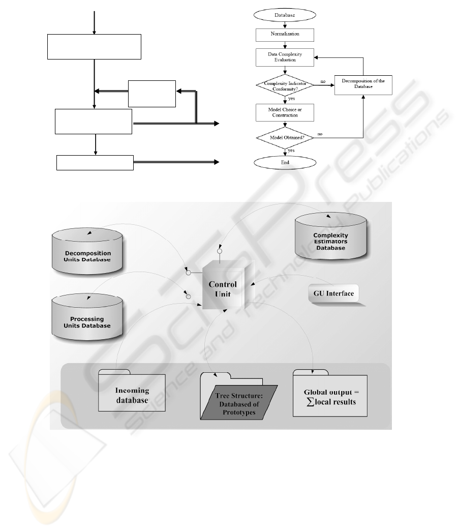
processing methods powered by a control engine an accessible by operator thought
Graphic User Interface.
Processing Results
Structure Construction
Learning Phase
Feature Space Splitting
NN based Models Generation
Preprocessing (Normalizing,
Removing Outliers, Principal
Com
p
onent Anal
y
sis
)
(PD) - Preprocessed Data Targets (T)
Data (D), Targets (T)
P – Prototypes NNTP - NN Trained Parameters
Operation Phase
Complexity
Estimation
Module
Fig. 1. Bloc scheme of T-DTS: Left – Modular concept, Right – Algorithmical concept.
Fig. 2. T-DTS software architecture.
Those three databases can be independently developed out of the main frame and
more important - they can be easily incorporated into T-DTS framework.
For example, SOM-LSVMDT [6] algorithm; witch is based on the same idea of
decomposition, can be implement by T-DTS by mean of LSVMDT [7] (Linear Sup-
port Vector Machine Decision Tree) processing method incorporation into PU data-
base.
20

The current T-DTS software (version 2.02) includes the following units and methods:
1. Decomposition Units:
• CN (Competitive Network)
• SOM (Self Organized Map)
• LVQ (Learning Vector Quantization)
2. Processing Units:
• LVQ (Learning Vector Quantization)
• Perceptrons
• MLP (Multilayer Perceptron)
• GRNN (General Regression Neural Network)
• RBF (Radial basis function network)
• PNN (Probabilistic Neural Network)
• LN
3. Complexity estimators are [3] based on the following criteria:
• MaxStd (Sum of the maximal standard deviations)
• Fisher measure.
• Purity algorithm
• Normalized mean distance
• Divergence measure
• Jeffries-Matusita distance
• Bhattacharyya bound
• Mahalanobis distance
• Scattered-matrix method based on inter-intra matrix-criteria [8]
• ZISC© IBM ® based complexity indicator [4]
3 ZISC Complexity Indicator
3.1 Complexity Estimation in T-DTS Framework
In this subsection we pass ahead of the possible question concerning the word “com-
plexity”. Let us highlight that in this part we are not focused on studying statistical
complexity as it is used in the areas of physics and informational theory. There are
different concepts of complexity which are depending on chosen language base, the
type of difficulty focused on the type of formulation desired within that language [9].
We have to mention a growing criticism concerning the term complexity, because it
has been misused without a proper definition [10].
Accordingly to T-DTS concept Fig. 1, complexity estimation module plays a key-role
in decomposition process, and so is essential in tree structure construction process.
There are two main problems:
• finding of the optimal threshold value for selected complexity estimating in-
dicator,
• lack of the universal complexity estimator (method of complexity estimat-
ing) that could be applied for any classification task independently of data
nature.
We define a task complexity as the amount of neurocomputer computational resource
that it takes to solve a classification problem [11].
21

Thus the complexity here is the limited supply of these resources (amount of neurons)
once the appropriate program (classification methods) is supplied. Our primary study
interest is in classification complexity in term of computational difficulty of neuro-
computer IBM © ZISC-036 ® hardware to obtain satisfactory learning and generali-
zation rates using RBF algorithm and adjusted initial parameters.
3.2 Complexity Estimating based on IBM© ZISC-036® Hardware
This complexity criterion is based on IBM © ZISC-036 ® neuro-computer hardware
which is a fully integrated circuit based on neural network paradigm [12]. It is a par-
allel neural processor based on the K-Nearest Neighbor (KNN) [13] and Reduced
Coulomb Energy (RCE) [14] algorithms. The principal idea for extracting informa-
tion about classification task complexity is linked to the limitation of resources (neu-
rons) of IBM © ZISC-036 ® neuron-computer.
We expect that a more complex problem will involve a more complex ZISC neural
network structure. The simplest neural network structure feature is the number n of
neurons created during the learning phase. The following indicator is defined, where
n is a parameter that reflects complexity:
m
n
Q =
,
0,1 ≥≥ nm
(1)
We suppose that there exists some function n = g(.) that reflects problem complexity.
The arguments of this function may be the signal-to-noise ratio, the dimension of the
representation space, boundary non-linearity and/or database size. In a first approach,
we consider only g(.) function’s variations according to m (database size) axis: g(m).
We suppose that our database is free of any incorrect or missing information.
On the basis on g(m), a complexity indicator is defined as follow:
m
mg
mQ
i
i
)(
)( =
0)(,1, ≥≥ mgm
i
(2)
We expect that for the same problem, as we enhance m, the problem seems to be less
complex: more information reduces problem ambiguity. On the other hand, for prob-
lems of different and increasing complexity, Q
i
indicator should have a higher value.
In order to estimate a task (sub-task) complexity we approximate Q
i
indicator and
figure the complexity ration out by the proposed method in [14].
In next section we discuss the results of the tests obtained by ZISC complexity es-
timator and compare them to the results of the others complexity estimators of T-DTS
framework.
4 Results and Discussion
In order to evaluate ZISC complexity estimator performance we have used for the
range of validation problems mentioned in the work [3]. There are:
1. Specific two-class 2D benchmark problems:
22
• 2 stripes simply separated by line X=0. Each stripe belongs to different
class.
• 10 stripes. Each of the class consists 5 stripes. The borders between
classes are lines X=b
i
(i = 1,2, … 9)
2. Tic-tac-toe endgame classification problems. The aim is to predict whether
each of 958 legal endgame boards for tic-tac-toe is won for `x'. This problem
is hard for the covering family algorithm, because of multi-overlapping [15]
that has a place.
3. Splice-junction DNA Sequences classification problem from Genbank 64.1
(ftp site: genbank.bio.net) has the following description:
• Number of Instances: 3190
• Number of Attributes: 62
• Missing Attribute Values: none
• Class Distribution:
1) EI: 767 (25%)
2) IE: 768 (25%)
3) Neither: 1655 (50%)
We used T-DTS in decomposition mode supposing that task must be divided into two
sub-tasks at least.
85.5
87.5
89.5
91.5
93.5
95.5
97.5
99.5
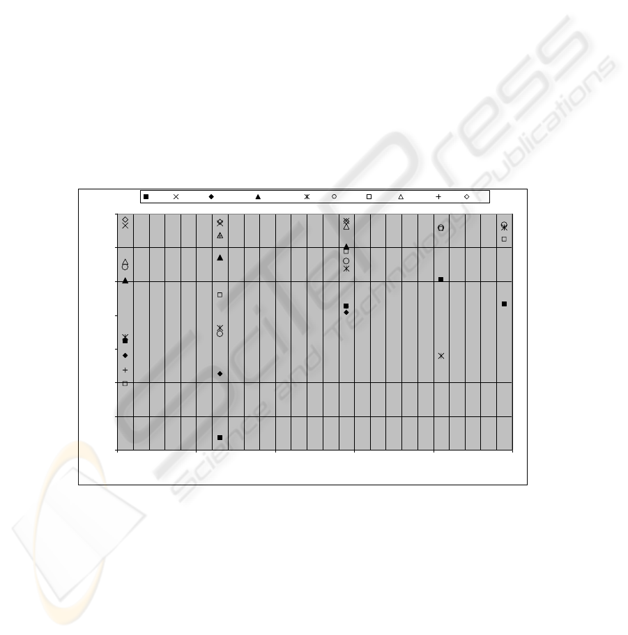
0.655 0.705 0.755 0.805 0.855 0.905
Threshold
Generalization rate (%)
Purity Mat Var Divergence Norm. Mean ZISC MaxS td Fisher Jef. Mat. Bhatt Mahal
Fig. 3. 2D-benchmark, two classes, 2-stripes. The vectors number - 2000. Learning database
50% (1000 vectors). DU - CN. PU – LVQ.
For each problem and chosen complexity estimation method the optimal decomposi-
tion threshold have been adjusted. For ZISC complexity estimator the initializing
intra-parameters have been also optimized. On Fig. 3 the X axis represents the de-
composition threshold ratio, on Y axis the Generalization rate for the whole range of
complexity estimation criteria.
23
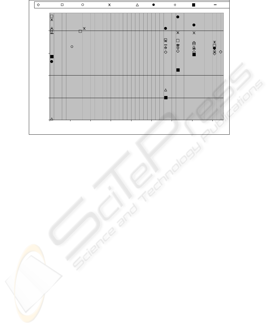
25.5
30.5
35.5
40.5
45.5
0.09 0.19 0.29 0.39 0.49 0.59 0.69 0.79 0.89
Threshold
Generalization rate
Purity GR Mat Var Divergence Norm. Mean ZISC Max St d Fisher Jef. Mat. Bhatt.
Fig. 4. 2D-benchmark, two classes, 10-stripes. The vectors number - 2000. Learning database
20% (400 vectors). DU - CN. PU – LVQ.
For two class’s benchmark within two sub zones, ZISC complexity indicator takes an
average position among the other complexity indicators; however for threshold 0.900
the ZISC based complexity estimator can achieve the maximal (e.g. the best) gener-
alization rate attaining approximately 99%. The result obtained for the other case (see
Fig. 4) spotlights the same conclusion: ZISC complexity indicator is not the worst
method among others. It is relevant to call attention to the fact that if the problem here
is already a same 2-D classification dilemma, the complexity has extremely been
increased (for 10-stripes variant). Moreover, the learning database’s size has been
reduced in order to check T-DTS generalization / decomposition ability within the
worst-case constraints. In fact, in such worst-case conditions, crop up from conjunc-
tion of intrinsic classification complexity and information leakage (emerging from
learning database reduced size) it is expectable to face such low generalization rate
(around 45%). Finally, the interesting result of Fig.4 highlights the ZISC (and more
generally, the “learning”) based complexity estimators’ main limit related to the re-
quirement of sufficient amount of training data.
For Tic-tac-toe highly overlapping problem (results of Fig. 5), ZISC complexity
estimator holds second position. Only Mahalanobis distance based measure of com-
plexity estimation has achieved better generalization rate than ZISC. However, con-
sidering the same test with a reduced learning database (including 20% of data), it is
interesting to note that, if the leader complexity estimator was Bhattacharyya bound
based criterion, again the second rank has been captured by ZISC based complexity
estimator.
24
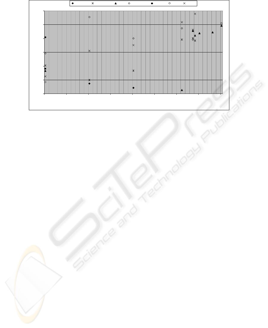
73
75
77
79
81
83
85
0.095 0.195 0.295 0.395 0.495 0.595 0.695 0.795 0.895
Threshold
Generalization rate
Mat Var 2 Norm Mean ZISC Max St. Dv. Jef. Mat Bhatt. Mahal
Fig. 5. Tic-tac-toe endgame problem. Number of vectors - 958. Learning database size 50%
(479 vectors). Decomposition unit - CN. Processing unit – MLP.
Another important note concerning the Tic-tac-toe end game problem is that in this
case, Purity and Divergence based indicators cannot be applied. In fact, based essen-
tially on clusters’ borders overlap, these indicators conclude on high complexity of
both problem and sub-problems, due to the high overlapping. As result, it is impossi-
ble to optimize thresholds for those criteria.
For Splice-junction DNA Sequences classification problem results are given in Fig. 6.
One can remark that ZISC based complexity estimator is a leader among the indica-
tors. Inapplicable indicators for this problem are: MaxStd (The sum of maximal stan-
dard deviation during decomposition process indicates problem as complex), Normal-
ized mean can not be applied because each vector consists 62 attributes and the com-
plexity ratio which is based on root square deviation indicates problem as a complex.
In this regard, there is no surprise why Fisher criterion is the worst one.
Summarizing the comparison of the indicators, we can state that ZISC complexity
indicator is matchless among the others. It is so, because ZISC based approach is not
sensitive to the number of attributes (of the input vector). For example (see Fig. 6)
ZISC complexity estimator for a threshold grater than 0.8 is the only indicator able to
provide correct feedback of complexity ratio to T-DTS. However, ZISC requires
optimization of the initializing internal parameters and moreover, ZISC estimation
complexity procedure is time-costly in comprising to the others.
Concerning the quality side of the obtained results for real-world problems (Tic-tac-
toe and DNA classification problem) we can conclude the following:
• for Tic-tac-toe endgame problem, T-DTS can reach 84% of generalization rate
for the Mahalanobis and Bhattacharyya criteria’s. With ZISC complexity esti-
mator we can achieve maximum of 82% generalization rate. Those results are
average in comparison to IBL family algorithms (Instanced Based Learning)
[15]. However some of IBL algorithms (as the IB3-CI algorithm) lead to better
results, they are specially adjusted for this problem.
25
• for DNA, we have obtained maximal generalization rate of 80% using ZISC es-
timator and this is the best among all other criteria’s. This result corresponds to
the results gained in the work [3].
56.95
61.95
66.95
71.95
76.95
81.95
0.09 0.19 0.29 0.39 0.49 0.59 0.69 0.79
Threshold
Generalization rate
ZISC GR Purity Norm. Mean Fisher Divergence Bhat Mahal Mat Var
Fig. 6. DNA Sequences problem. M=1900. Learning DB size - 20%. DU - CN. PU – MLP.
Finally, one can remark that the generalization rate of 82%, reached by ZISC based
T-DTS for Tic-Tac-Toe end problem, is very close to 84% (obtained by Mahalanobis
and Bhattacharyya based T-DTS). So it presents quite high generalization rates. For
DNA sequence classification, ZISC based T-DTS, overcome all other complexity
based T-DTS. In these last two cases, the representation space has a high dimension.
One can conclude that ZISC based T-DST is an appealing candidate for solving high
dimension problems. We are conducting other experiments in order to check this
hypothesis.
5 Conclusions
Incorporating a new complexity estimator, based on ZISC neuro-computer, the goal
was to check the performance of T-DTS regarding other various complexity estima-
tion modules, already implemented in T-DTS framework. We have used the T-DTS
framework to solve three classification problems. The proposed complexity estima-
tion criterion has been evaluated using as well benchmark as real-world problems.
We have shown that the ZISC based complexity estimator allows the T-DTS based
classifier to reach better learning and generalization rates. We have also illustrated
that this indicator is matchless for classification tasks relating problems with high
dimension feature space. In this case, statistical based complexity indicators fail to
work. However, the ZISC based complexity estimator requires sufficient amount of
26

training data which is a general operation condition (requirement) for all artificial
learning based techniques.
The main future perspective of this work is related to T-DTS automatic optimization
of and to the extension of database decomposition methods.
References
1. Bouyoucef E., Chebira A., Rybnik M., Madani K.: Multiple Neural Network Model Gen-
erator with Complexity Estimation and Self-Organization Abilities: International Scientific
Journal of Computing (2005) Vol. 4. Issue 3. 20–29.
2. Rybnik M.: Contribution to the Modeling and the Exploitation of Hybrid Multiple Neural
Networks Systems: Application to Intelligent Processing of Information, PhD Thesis, Uni-
versity Paris XII, LISSI (2004)
3. Bouyoucef E.: Contribution à l’étude et la mise en œuvre d’indicateurs quantitatifs et
qualitatifs d’estimation de la complexité pour la régulation du processus d’auto
organisation d’une structure neuronale modulaire de traitement d’information, PhD Thesis
(in French), University Paris XII, LISSI (2006)
4. Budnyk I., Chebira A., Madani K.: Estimating Complexity of Classification Tasks Using
Neurocomputers Technology: International Scientific Journal of Computing (2007)
5. Madani M., Rybnik M., Chebira A.: Data Driven Multiple Neural Network Models Genera-
tor Based on a Tree-like Scheduler: Lecture Notes in Computer Science edited Mira. J.,
Prieto A.: Springer Verlag (2003). ISBN 3-540-40210-1, 382-389.
6. Mehmet I. S., Bingul Y., Okan K. E., Classification of Satellite Images by Using Self-
organizing Map and Linear Support Vector Machine Decision Tree, 2nd Annual Asian
Conference and Exhibition in the field of GIS, (2003).
7. Chi H., Ersoy O.K., Support Vector Machine Decision Trees with Rare Event Detection,
International Journal for Smart Engineering System Design (2002), Vol. 4, 225-242.
8. Fukunaga K.: Introduction to statistical pattern recognition, School of Electrical Engineer-
ing, Purdue University, Lafayette, Indiana, Academic Press, New York and London, (1972).
9. Edmonds B., What is Complexity? - The philosophy of complexity per se with application
to some examples in evolution: Heylighen F. & Aerts D. (Eds. 1999): The Evolution of
Complexity, Kluwer, Dordrecht.
10. Feldman D.P., Crutchfield J.P.: Measure of statistical complexity: Why? Phys. Lett.(1998)
A 238: 244-252.
11. Budnyk I., Chebira A., Madani K.: ZISC Neural Network Base Indicator for Classification
Complexity Estimation, ANNIIP (2008), 38-47.
12. Madani K., Chebira A.: Data Analysis Approach Based on a Neural Networks Data Sets
Decomposition and it’s Hardware Implementation, PKDD, Lyon, France (2000).
13. Dasarathy B.V. editor (1991) Nearest Neighbor (NN) Norms: NN Pattern Classification
Techniques. ISBN 0-8186-8930-7
14. Park. J., Sandberg J. W.: Universal Approximation Using Radial Basis Functions Network,
Neural Computation (1991) Volume 3, 246-257.
15. Aha. D. W., Incremental Constructive Induction: An Instance-Based Approach. In Proceed-
ings of the Eight International Workshop on Machine Learning. Morgan Kaufmann (1991),
117-121.
27
