Situational Reasoning for Road Driving in an Urban
Environment
Noel E. Du Toit, Tichakorn Wongpiromsarn, Joel W. Burdick and Richard M. Murray
California Institute of Technology, Division of Engineering and Applied Science
1200 E. California Blvd, Pasadena, CA 91125, U.S.A.
Abstract. Robot navigation in urban environments requires situational reason-
ing. Given the complexity of the environment and the behavior specified by traf-
fic rules, it is necessary to recognize the current situation to impose the correct
traffic rules. In an attempt to manage the complexity of the situational reasoning
subsystem, this paper describes a finite state machine model to govern the sit-
uational reasoning process. The logic state machine and its interaction with the
planning system are discussed. The approach was implemented on Alice, Team
Caltech’s entry into the 2007 DARPA Urban Challenge. Results from the qual-
ifying rounds are discussed. The approach is validated and the shortcomings of
the implementation are identified.
1 Introduction
The problem of robot navigation in urban environments has recently received substan-
tial attention with the launch of the DARPA Urban Challenge (DUC). In this competi-
tion, robots were required to navigate in a fully autonomous manner through a partially
known environment populated with static obstacles, live traffic, and other robots. In or-
der for the robot to complete this challenge, it needed to drive on urban roads, navigate
intersections, navigate parking lots, drive in unstructured regions, and even navigate un-
structured obstacle fields. Since the environment was only partially known prior to the
race, the robot needed to rely on sensory information to extract the world state, which
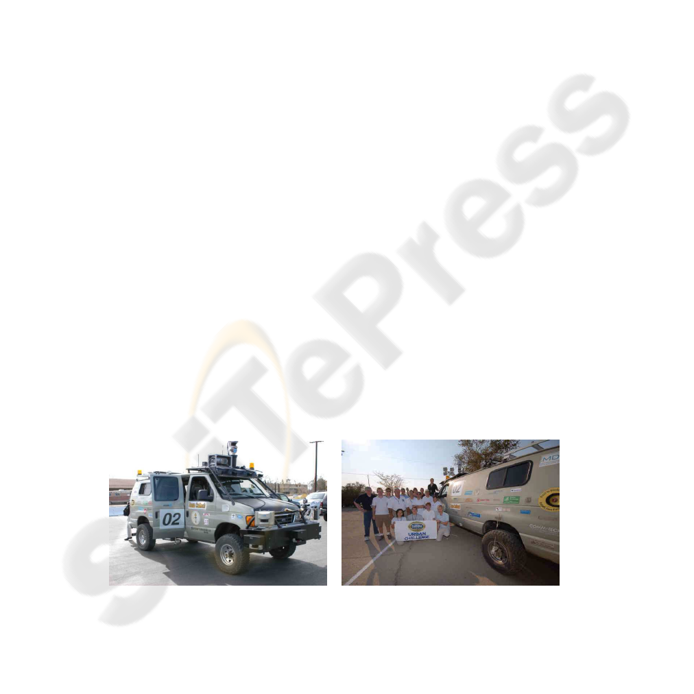
Fig.1. Alice (left), Team Caltech’s (right) entry in the 2007 DARPA Urban Challenge.
E. Du Toit N., Wongpiromsarn T., W. Burdick J. and M. Murray R. (2008).
Situational Reasoning for Road Driving in an Urban Environment.
In Proceedings of the 2nd International Workshop on Intelligent Vehicle Control Systems, pages 30-39
Copyright
c
SciTePress

introduces additional uncertainty into the problem. Furthermore, lack of exact knowl-
edge about the robot’s location and the state and intent of dynamic obstacles introduced
further uncertainty. Lastly, the robot needed to obey California traffic rules or exhibit
human-like behavior when this was not possible.
The urban component of the problem had two effects on the robotic planning prob-
lem: first it introduced some structure into the environment that could be used during
the planning process. Second, the traffic rules associated with urban driving forced the
robots to exhibit specific behaviors in specific situations. These behaviors are at a high
level associated with the driving task that is being executed, which include, for example,
driving on a road versus driving in a parking lot. While executing a driving task, it is
necessary for the vehicle’s control system to reason about which traffic rules are appli-
cable at each instant. It was not sufficient to obey all the rules all the time, but in some
cases constraints needed to be relaxed for the robot to make forward progress. This rea-
soning module is what is presented in this work. A related aspect of urban driving is
intersection handling [1] and is not discussed here.
Prior work has attempted to solve the problem of reasoning about the robot’s correct
driving behavior. Most of the work has been related to highway driving, and deciding
when a maneuver such as a lane change or emergency maneuver is in order [2–5]. One
practical hurdle is managing the complexity of the decision-making module [2] which
must decide which rules to enforce and which actions to take. Another problem is tak-
ing uncertainty about the situation into account. Sukthankar et al. [2] implemented a
scheme based on a voting system, called polySAPIENT. Different traffic objects in the
environment (for example another car, an exit on the highway, etc.) would vote for
the appropriate action. Using a mitigation scheme, the best action was chosen. Unsal
et al. [3] used automata theory for longitudinal and lateral control of the vehicle, and
implicitly chooses the best action. Gregor and Dickmanns [4] used a finite state ma-
chine (FSM) to decide. Niehaus and Stengel [5] explicitly account for uncertainty in a
probabilistic fashion, and use a heuristic method to select the best action.
The main contribution of this paper is the design of a decision module for a robot
navigating an urban environment. To manage complexity, this module does not attempt
to explicitly reason about all aspects of the environment, but instead makes use of infor-
mation generated by the path-planning module to guide decisions. The decision module
was implemented on Alice, the Team Caltech entry into the DUC (see figure 1). Results
obtained during successful DUC qualifying runs are presented. The paper is structured
as follows: the overall planning approach is briefly reviewed in section 2, before fo-
cussing on reasoning in the logic planner (section 3). An example is given to illustrate
usage. Lastly, some results from the qualifying runs for the DUC are presented, with a
discussion, recommendations and future work.
2 Overview of Planning Approach
The planning problem involved three driving tasks: road driving, off-road driving, and
parking lot navigation. In an attempt to modularize the system for rapid development,
the problems of sensing, planning, and control were separated. The planning problem
itself was divided into three layers (see figure 2), following the hierarchical architec-
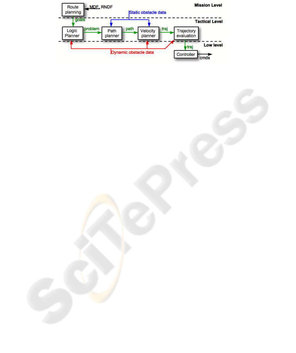
Fig.2. Planning architecture showing 3 layers used for planning process.
ture dictated by the contingency management approach that was adopted for overall
management of Alice’s activities [6].
At the mission level, it was necessary to generate a route through the road net-
work, as defined by DARPA through the Road Network Definition File (RNDF). The
route planner would specify a sequence of road segment goals to be completed, which
would be passed to the tactical planning layer. The tactical planner was responsible for
generating a trajectory to some intermediate goal (e.g., a position at the end of a road
segment). The reasoning methodology used by the tactical planner is the focus of this
paper. The trajectory generated in the tactical planner was in turn passed to a low-level
trajectory-following controller, which is documented in [7].
The tactical planner consisted of four parts:
Logic Planner: The logic planner was the reasoning module of the robot. This module
had two functions: reasoning about the current traffic situation, and reasoning about
intersections [1]. This planner was implemented as a set of finite state machines (FSMs)
and would set up a planning problem to be solved. Reasoning about the current traffic
state is the focus of this paper.
Path Planner and Velocity Planner: The trajectory planning problem was separated
into a spatial and a temporal planning problem in order to simplify these planning prob-
lems, and to satisfy the real-time requirement of the planner. Separate path planners
were implemented for the three different driving tasks. These path planners were re-
sponsible for solving the 2-D spatial path planning problem, accounting for the static
component of the environment. The velocity planner time-parameterized the path to ob-
tain a detailed trajectory. This velocity planner adjusted the robot’s speed for stop lines
along the path, static obstacles on or near the path, the curvature of the path, and the
velocities of dynamic obstacles.
Trajectory Analysis (and Prediction): Navigating in urban environments requires the
incorporation of the (predicted) future states of dynamic obstacles in the planning prob-
lem. Prediction involves two estimation processes: predicting the behavior of the dy-
namic obstacle, and predicting the future states of the dynamic obstacle. This informa-
tion can be compared to the robot’s planned trajectory to detect future collisions. The
generation and use of prediction information will be presented elsewhere.
An important part of the navigation problem was contingency management and in-
ternal fault handling.The hierarchical planning architecture lined up well with the conti-
gency management philosophy that was adopted. The Canonical Software Architecture

Fig.3. Example problem: the travel lane of the robot is blocked. Using the failure of the path
planner, the logic planner infers that the lane is blocked and relaxes the lane keeping constraint.
This allows the robot to execute a passing maneuver.
was adopted, where each module handled its internal faults and the failures propagated
from the lower-level modules. When the module could not reach its goal, it would fail
to the level above, which would adjust the goal. A complimentary, detailed discussion
of contigency management has been presented in [6].
3 Situational Reasoning with the Logic Planner
Situational reasoning is necessary to impose both the traffic rules, and the correct behav-
ior when rules need to be relaxed. For the highway driving case, the environmentis very
structured, and the behavior of the other dynamic agents that might be encountered by
the vehicle is relatively constrained, yet the complexity of the reasoning modules was
a problem. One reason for this complexity is because these modules attempt to reason
about all components of the environment abstractly. For example, the reasoning module
would need to obtain a list of obstacles in the robot’s vicinity, and reason about their
position (e.g., in lane) in the environment, the context (e.g., static obstacle blocking
the lane) and how that may affect the robot (e.g., need to change lanes). Alternatively,
much information is obtainable from the path and velocity planners, and could be used
to guide the decision process. For example, when the path planner could not find a
collision-free path, an obstacle must be blocking the lane. This information could be
returned to the reasoning module via a status message, SM, to be used in the decision
making. Decision making was avoided while things were running smoothly. For further
simplicity, the reasoning module was reduced to a finite state machine (FSM).
Example: To understand the reasoning approach, it is useful to look at an example
(see figures 2 and 3). Consider the case of the robot driving down a two-lane, two-way
road segment.
Cycle k-1: From the previous planning cycle, no problem was detected by any com-
ponent of the tactical planner. Imagine now that a static obstacle is detected in the
robot’s driving lane.
Cycle k: The path planner cannot find a collision-free path that stays in the lane
and reaches the goal location. The planner reports the status: SM = COLLP AT H ,
and encodes the position of the obstacle in the path structure. From SM, the velocity
planner observes the obstacle and plans to bring the vehicle to a stop.
Cycle k+1: The logic planner evaluates SM, and observes that the path contains a
collision with a static obstacle. Given the current constraint to stay in the lane, the goal
cannot be reached and the lane must be blocked. The appropriate behavior for the robot
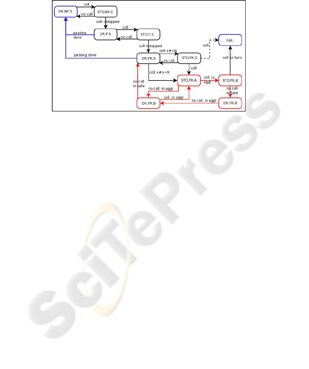
Fig.4. The logic planner finite state machine for driving in a road region.
would be to drive up to the obstacle and come to a complete stop. Now jump i cycles
ahead, to where the robot is stopped.
Cycle k+i+1: Once the robot is stopped, the reasoning module relaxes the constraint
to stay in the lane. The path planner searches the adjacent lane. No collision is reported
for this new planning problem and the robot is allowed to pass.
Logic Planner: The logic planner was implemented as a finite state machine. For
the road navigation, the machine consisted of 10 states denoted by ([M,F,C]). The states
constisted of a mode (M), a flag (F), and an obstacle clearance requirement (C). The
state machine is illustrated in figure 4. During urban navigation, the robot must interact
with static and dynamic obstacles. For planning, the static obstacles required an ad-
justment of the spatial plan, where as dynamic obstacle required an adjustment of the
robot’s velocity. Separating the spatial and velocity planning and encoding the dynamic
obstacle information on the path, the velocity planner alone could account for the nom-
inal interaction with the dynamic obstacle (such as car following), and the logic did not
explicitly have to deal with this problem.
The modes included driving (DR) and stopping for obstacles (STO). The flags in-
cluded no-passing (NP), passing without reversing (P), and passing with reversing (PR).
The obstacle clearance-modes included the nominal, or safe, mode (S), an aggressive
mode (A), and a very aggressive, or bare, mode (B). The state machine can be divided
into trying to handle the obstacle while maintaining the nominal clearance ([·,·,S]), and
being more aggressive. The second option was only invoked when the first failed, and
safe operation was guarenteed by limiting the robot speed in these aggressive modes.
The nominal state for road driving, [DR,NP,S], was to allow no passing, no re-
versing, and the nominal obstacle clearance, termed safety mode. With no obstacles
blocking the desired lane, the logic state remained unchanged. When a static obstacle
was detected, the path planner would: (i) find a path around the obstacle while staying
in lane, (ii) change lanes to another legal lane (if available), or (iii) report a path with

a collision. For case (iii), the logic planner would know that a collision free path was
not available from the status message (SM), and would switch into obstacle handling
mode.
The correct behavior when dealing with a static obstacle was to drive up to it, com-
ing to a controlled stop [STO,NP,S] (refer to figure 4). If at any time the obstacle dis-
appeared, the logic would switch back to the appropriate driving mode. Once the robot
was at rest, the logic switched to driving mode, while allowing passing into oncoming
lanes of traffic [DR,P,S]. If a collision free path was obtained, then the robot would
pass the obstacle and switch back to the nominal driving state once the obstacle had
been cleared. If a collision free path did not exist, then the logic would again make sure
that the robot was stationary before continuing [STO,P,S]. At this point, either (i) the
robot was too close to the obstacle, (ii) there was a partial block and by reducing the
obstacle clearances the robot might squeeze by, or (iii) the road was fully blocked. The
first case was considered by switching into a mode where both passing and reversing
was allowed [DR,PR,S]. If a collision free path was found, the passing maneuver was
performed. If a collision was detected and persisted, the robot would again be stopped
[STO,PR,S]. At this point, reducing the obstacle clearance and proceeding with caution
was considered.
Given the size of the robot (the second largest robot in the 2007 DUC), a major
concern was maneuvering in close proximity to static obstacles. To curb this problem,
it was desirable to reduce the required obstacle clearances. First the robot switched
to aggressive mode, [STO,PR,A]. If a collision free path was found, the robot would
drive in this mode [DR,PR,A]. As soon as a path was found that satisfied the nominal
obstacle clearance, the logic switched back to [DR,PR,S]. If the robot could not find a
collision free path while in aggressive mode, it would reduce the obstacle clearances
even further by switching to bare mode [STO,PR,B]. If a path was found, it would
drive in this mode [DR,PR,B] until a path was found that did not require this mode.
The logic would then switch back to the aggressive mode [DR,PR,A]. If no collision
free path could be found, even in bare mode, the conclusion was that the road must be
blocked. At this point, the tactical planner could not complete the segment-levelgoal. In
accordance with the contigency management strategy, the tactical planner sent a failure
to the route planner, which replanned the route. If the robot was on a one-way road, the
route-planner would allow the robot to enter off-road mode, as a last resort.
Since reversing was allowed, it was possible for the robot to get stuck in a cycle of
not finding a path [STO,PR,S], then backing up and finding a path [DR,PR,S], driving
forward and detecting a collision, backing up again, etc. In an attempt to avoid this cycle
and others like it, some transitions were created to exit these loops (from [DR,PR,S])
as part of contigency management.
4 Results and Discussion
The tactical planner, and logic planner, was implemented on Alice, a modified Ford
E350 van (see figure 1). The robot was equipped with 24 CPUs, 10 LADAR units, 5
stereo camera pairs, 2 radar units, and an Applanix INS to maintain an estimate of its
global position.
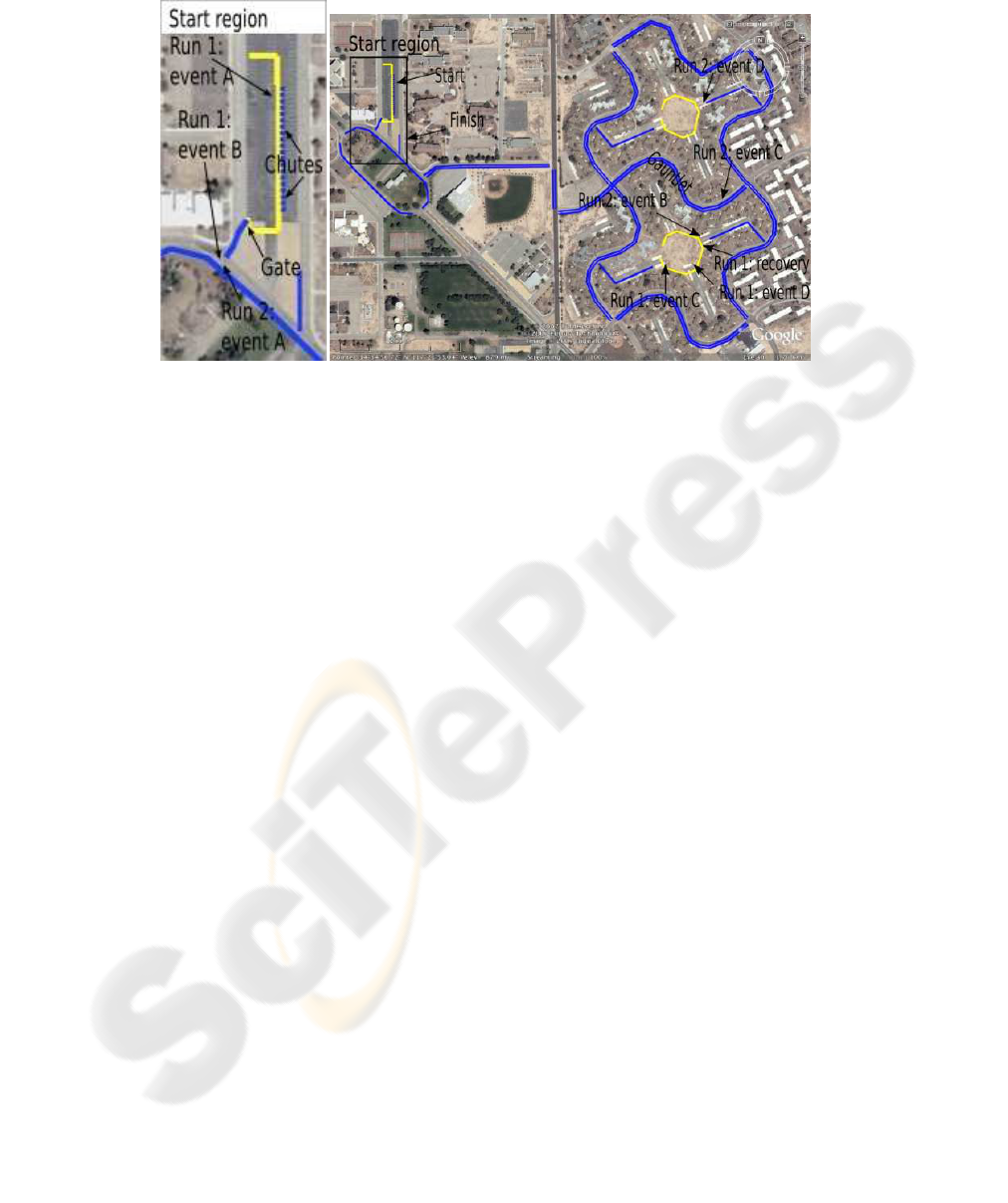
Fig.5. RNDF and aerial image of Area B.
The NQE consisted of three test areas, which tested different aspects of urban driv-
ing. The course of interest here is area B, for which the RNDF, overlayed with aerial
imagery, is given in figure 5. The course consisted of approximately 2 miles of urban
driving without live traffic and tested the robot’s ability to drive on roads, in parking
areas, and in obstacle fields. The course was riddled with static obstacles. The robots
started in the starting chutes, which were short lane segments, lined with rails. The robot
would drive into an open area and proceed to a gate. The gate led to a one-way road,
lined with rails, which in turn led to an intersection and the course. The robots would
then proceed around a traffic circle and make its way to the parking zone (southern oc-
tagonal region). Once through this parking lot, the robot passed through the ‘gauntlet’,
and made its way to the northern zone (obstacle field). From there, it would make its
way back to the finish (next to the start area). The results are presented next, followed
by a discussion.
4.1 Run 1
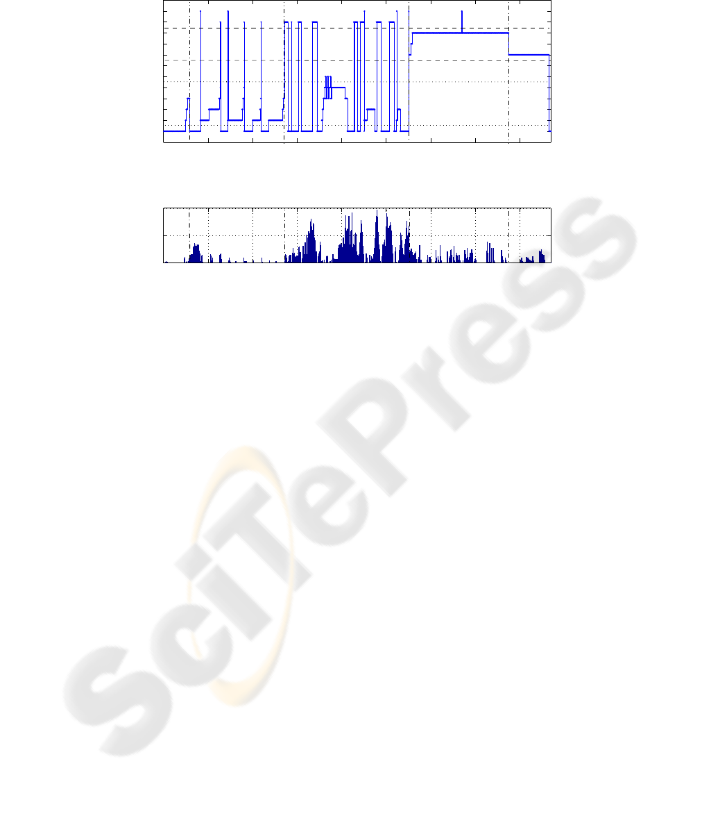
The logic states and velocity profile for run 1 are presented in figures 6 and 7, respec-
tively. Four events are indicated on these figures, and the corresponding locations are
shown in figure 5. The robot had difficulty exiting the start area (events A and B), but
made rapid progress before getting stuck in the parking lot (event C) and was manually
reset (event D). It still could not exit the parking area and was eventually recovered
from the parking area.
The robot was in the nominal driving state ([DR,NP,S]) only 29.5% of the run (see
figure 6). Since the robot got stuck in the parking area (event C and onwards) and ended
up spending 34.3% of the run there, it is more useful to consider the logic data up to
event C. The robot spend 44.3% of the run up to event C in the nominal driving state,
which was still a low number. The logic switched out of the nominal state 8 times to deal
with obstacles, of which 5 were in the start area. 42.8% on the run (up to the parking
0 200 400 600 800 1000 1200 1400 1600
NP,S
P,S
PR,S
PR,A
PR,B
OFFROAD
UTURN
SAFE
AGGR
BARE
ST_INT
PAUSE
A
C
Exception handling
Obstacle handling
Nominal driving
Road region
Zone region
B
D
Fig.6. Logic planner states during run 1 of NQE area B.
0 200 400 600 800 1000 1200 1400 1600
0
5
10
Time [s]
Velocity [m/s]
A
B
D
C
Fig.7. Velocity profile during run 1 of NQE area B.
area) was spent dealing with obstacles - 30.2% in the nominal obstacle clearance mode,
and 12.6% in the more aggressive modes. It also switched out of intersection-handling
mode due to static obstacles 3 times and was in exception handling mode 0.65% of the
total run.
The robot spent the first 9 minutes in the start area, where it needed to travel
through a gate and an alley (event B). The logic correctly switched into the aggressive
modes since the alley was too narrow for the robot to pass through while maintain-
ing the nominal obstacle clearance. Unfortunately, the implementation of the switching
to intersection-handling mode was lacking, and the obstacle clearance would get reset
causing the path-planner to fail again. This happened 3 times in the start area, and the
robot was stationary much of the time in this area (see figure 7). The robot swiched to
the aggressive modes, and eventually to a failure mode, later in the run (around 700 s)
due to a misallignment of the road and the RNDF. The robot got stuck in the parking
area since it again could not maintain the necessary obstacle clearances and complete
the goal. In this case, even the most aggressive mode was not sufficient.
The team realized that, in order to compete, it needed to adjust it’s strategy. It
was necessary to be more aggressive around static obstacles, but still maintain op-
erational safety. It was decided to reduce the nominal obstacle clearance to the bare
value by default, thereby collapsing the logic for changing this distance in the logic
planner. That meant removing the connections between [DR,PR,S]→[STO,PR,A] and
[STO,PR,S]→[STO,PR,A] (see figure 4). A connection (shown with a dashed arrow)
was added from [STO,PR,S]→[FAIL]. For safety, the planner relied on the velocity
planner to slow the robot near obstacles.

0 200 400 600 800 1000 1200 1400
NP,S
P,S
PR,S
OFFROAD
UTURN
ZONE
ST_INT
PAUSE
Time [s]
D
C
B
A
Obstacle handling
Exception handling
Road region
Zone region
Nominal driving
Fig.8. Logic planner states during run 2 of NQE area B.
4.2 Run 2
The logic states for the second attempt are shown in figure 8. The robot was able to
complete the run in a little over 23 minutes. It effortlessly exited the start area (event
A), and drove up to and through the parking area (event B). Next, it navigated the
‘gauntlet’ (event C) successfully, before driving through the obstacle field (event D),
and on to the finish area.
The robot spent 61.6% of the run in the nominal driving mode, and dealt with obsta-
cles for 11.6% of the time. The robot switched out of the nominal driving mode 4 times
to deal with obstacles. It also spent 16.5% of the time in intersection handling mode (14
intersections), and spent 7.93% of the run performing the parking maneuver. The robot
spent 1.73% of the run navigating the obstacle field, and had no exceptions.
The time spent in obstacle mode was still worrisome. During the navigation of the
‘gauntlet’, the obstacles were so close together (longitudinally) that the function esti-
mating the completion of the passing maneuver was insufficient. Thus, the robot re-
mained in passing mode during most of this section.
4.3 Discussion
The notion of using the path planner capabilities to assist in the decision making pro-
cess worked very well, even though the implementation was not perfect. The significant
improvement in performance from run 1 to run 2 was due to the effective reduction in
size of the robot. Some implementation shortcoming have been mentioned, and are
summarized here. It is important to note that these shortcomings are often artifacts of
other parts of the system. The logic for switching to intersection handling was fragile
since the obstacle clearance mode was reset. Also, estimating whether a passing maneu-
ver was complete was not robust. This was complicated by the path planning approach
used. One shortcoming of the approach was not explicitly accounting for uncertainty in
the decision process. It had been intended to extend the logic to account for this, but due
to the time constraints it was not possible. However, by using the planner components
to assist in the decision making, this shortcoming was largely mitigated.
5 Conclusions and Future Work
An approachto situational reasoning for driving on roads in urban terrain was described.
In an attempt to manage the complexity of the reasoning module, knowledge from the

path planner was used and the reasoning module was implemented as a finite state ma-
chine. This module was only invoked when the planner failed to find a solution while
satisfying all the constraints imposed by the traffic rules. The reasoning module was
implemented as part of a complete (and complex) autonomous system, developed for
urban navigation. The performance of the module was discussed based on the results of
the two runs in area B during the DUC NQE. The module imposed the correct behavior
on the robot in most cases. The failures were a result of the implementation and the size
of the robot. Uncertainty was handled implicitly through the use of the planner compo-
nents to assist in the decision making. Future work includes extending this approach to
explicitly account for uncertainty during the decision process.
Acknowledgements
The work presented here is the culmination of many members of Team Caltech, espe-
cially: Vanessa Carson, Sven Gowal, Andrew Howard, and Christian Looman.
This work was supported in part by the Defense Advanced Research Projects Agency
(DARPA) under contract HR0011-06-C-0146, the California Institute of Technology,
Big Dog Ventures, Northrop Grumman Corporation, Mohr Davidow Ventures, and Ap-
planix Inc.
References
1. Looman, C.: Handling of Dynamic Obstacles in Autonomous Vehicles. Master’s thesis, Insti-
tut f¨ur Systemdynamik (ISYS), Universit¨at Stuttgart, (2007)
2. Sukthankar, R., Pomerleau, D., Thorpe, C.: A distributed tactical reasoning framework for
intelligent vehicles. SPIE: Intelligent Systems and Advanced Manufacturing, October, (1997).
3. Unsal, C., Kachroo, P., Bay, J. S.: Multiple Stochastic Learning Automata for Vehicle Path
Control in an Automated Highway System IEEE Transactions on System Man, and Cybernet-
ics, Part A: Systems and Humans, January, (1999).
4. Gregor, R., Dickmanns, E. D.: EMS-Vision: Mission Performance on Road Networks. Pro-
ceedings of the IEEE Intelligent Vehicles Symposium, (2000).
5. Niehaus, A. Stengel, R. F.: Probability-based decision making for automated highway driving.
IEEE Transactions on Vehicular Technology, Volume 43, p. 626-634, August, (1994)
6. Wongpiromsarn, T., Murray, R. M.: Distributed Mission and Contingency Management for
the DARPA Urban Challenge. Submitted to: International Workshop on Intelligent Vehicle
Control Systems, IVCS (2008)
7. Linderoth, M., Soltesz, K., Murray, R. M.: Nonlinear lateral control strategy for nonholonomic
vehicles. In: Proceedings of the American Control Conference. (2008) Submitted.
