A MATHEMATICAL FORMULATION OF A MODEL FOR
LANDFORM ATTRIBUTES REPRESENTATION FOR
APPLICATION IN DISTRIBUTED SYSTEMS
1
Leacir Nogueira Bastos,
1
Rossini Pena Abrantes and
2
Brauliro Gonçalves Leal
1
Informatics Department, Viçosa Federal University, PH Rolfs Avenue, Viçosa, Brazil
2
INTEC Group Researcher, Brazil
Keywords: Mathematical Modeling of Landform Attributes, Distributed Processing, Internet, Nonlinear Regression,
Polynomial Estimation.
Abstract: This study presents a methodology based on nonlinear regression for landform attributes representation. The
equations to estimate the parameters of a two-dimensional polynomial are shown and, for testing the
methodology, it was used the data from landform attributes of the state of Minas Gerais (Brazil) obtained by
the Digital Elevation Model (DEM) in GTOPO30 project. They form a regular grid, with spacing of
approximately 900m. The presented methodology can be used to minimize time of sending landform
attributes information through network, to minimize space by storing the parameters of the estimated
polynomial, and to make possible the process distribution of the polynomial coefficients calculations to
different CPUs over internet network.
1 INTRODUCTION
The increased efficiency and reliability of computer
networks (Fowler, 2005), as well as the
popularization of the Internet, have generated new
opportunities for applications development. Now,
with the growing number of connected computers in
the Internet (Zakon, 2006), it is possible to distribute
applications, using communication infrastructure,
without great efficiency problems. An application
that has access to the resources of the Internet can
use the services as HTTP, SMTP, POP3, FTP, for
updating through remote servers (Tanenbaum,
2002).
In Geo-informatics, there is an area called
Numerical Model of Surface that treats the
mathematical representation of landforms (INPE,
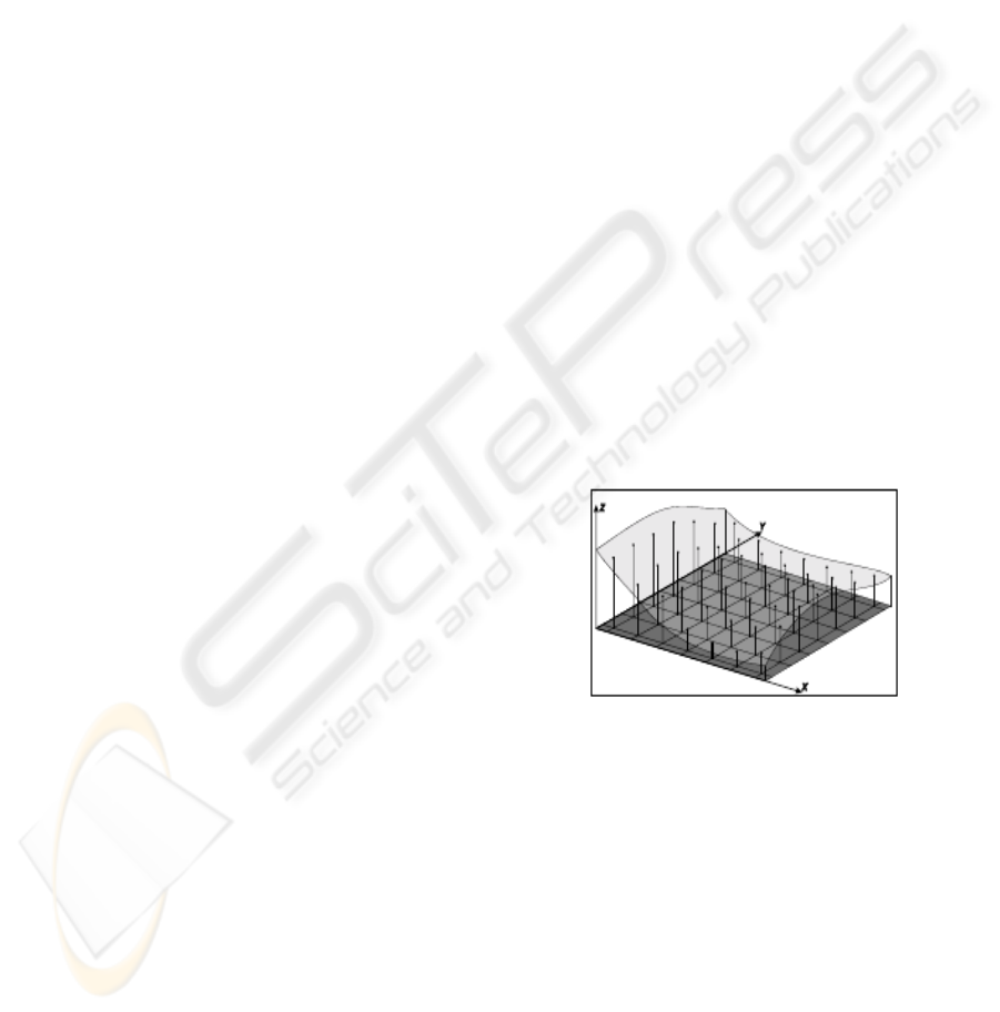
2001). One of the numerical models most common
used is the Regular Grid Model whose function is to
generate a grid starting from a group of elevation,
longitude and latitude points as in Figure 1.
Figure 1: Regular Grid Model.
This grid can be generated by point interpolation
for a polynomial regression model that adjusts a
two-dimensional polynomial which best represents
the landform attributes of an area (Burrough, 1986)
(Ervin and Hasbrouck, 2001). The regression
analysis is a statistical instrument often used in
science. Its common use is to make possible the
description of a phenomenon by means of a
mathematical model (equation), based on a data
sample. Graphically, it is equivalent to identify the
curve or mathematical surface that best adjusts to the
points in a dispersion diagram. The mathematical
models of regression are based in three statistical
assumptions: a) the relationship among the
184
Nogueira Bastos L., Pena Abrantes R. and Gonçalves Leal B. (2008).
A MATHEMATICAL FORMULATION OF A MODEL FOR LANDFORM ATTRIBUTES REPRESENTATION FOR APPLICATION IN DISTRIBUTED
SYSTEMS.
In Proceedings of the Fourth International Conference on Web Information Systems and Technologies, pages 184-189
DOI: 10.5220/0001527901840189
Copyright
c
SciTePress

dependent and independent variables is deterministic
instead of stochastic; b) the error measurements are
random, following the normal distribution, average
zero and constant variance; and c) the explanatory
variables don't show correlation among themselves
(Seber and Wild, 2005). This technique of landform
attributes representation has some advantages over
other techniques, basically by representing the
landform attributes by mathematical equations
instead of images, latitude, longitude and elevation
coordinates, or map of elevation levels. One of the
advantages is the significant reduction of the amount
of necessary information to represent the landform
attributes of a certain area, since, with the regression
technique, the landform attributes of an entire area
can just be represented through the coefficients of
two-dimensional polynomial. By the polynomial
representation it is possible to generate images with
different resolution levels because, with a
polynomial function, we may generate as many
points as needed. Besides these advantages, there is
a possibility to apply, on the polynomial, several
mathematical operations, such as finding the
maximal and minimal point, derivation, etc.
However, the technique of polynomial regression
has some disadvantages too, since the complexity
and the computational power demanded in obtaining
such polynomial is very high and sometimes
impractical.
For that reason the objective of this article is to
present a methodology designed to make possible
the distribution of the necessary processing to
compute a two-dimensional polynomial that
represents the landform attributes of an area and, as
an example, we use the area of the state of Minas
Gerais, in Brazil, located in the Southeastern area of
the country. Some estimative calculations, presented
in this article, show that the necessary time of
centralized processing to estimate such a polynomial
is prohibitive, being in order of dozens of
uninterrupted years of processing.
2 MATHEMATICAL METHOD
In this work we present a methodology for landform
attributes representation using the method of
nonlinear regression to adjust a two-dimensional
polynomial. The regression analysis is a statistical
instrument very used in science. Its frequent use is
due to the fact of making possible the description of
phenomena through mathematical models from a
data sample. Graphically, it is equal to identify the
curve or mathematical surface that best adjusts to the
points in a dispersion diagram. The mathematical
models of regression are based on three statistical
facts: a) the relationship among the dependent and
independent variables is deterministic instead of
stochastic; b) the errors are random with normal
distribution, average zero and constant variance; and
c) the explanatory variables don't present correlation
among themselves (Seber and Wild, 2005).
When a mathematical model of regression is
used, the most used method of estimating the
parameters is the Least Squares Method which
consists of estimating a function to represent a group
of points, minimizing the square of the deviations
(Nobel and Daniel, 1986). Considering a group of
geographic coordinates (x, y, z), representing
longitude, latitude, and elevation of each point,
respectively, we may take an estimate elevation
function
),(
ˆ
yxfz
=
of these points. A
polynomial of degree r in x and degree s in y can be
given, according to Equation 1, and the estimated
error ε
ij
is given by Equation 2 where 0 ≤ i ≤ m and
0 ≤ j ≤ n.
∑∑
==
==
r
k
s
l
l
j
k
iklji
yxayxfz
00
),(
ˆ
(1)
ijijij
zz
ˆ
−
=
ε
(2)
The coefficients a
kl
(k = 0, 1, ..., r, l = 0, 1, ..., s)
that minimize the errors of the estimated function
f (x, y) can be obtained by solving Equation 3 for c =
0, 1, ..., r and d = 0, 1, ..., s.
0=
∂
∂
cd
a
ξ
(3)
where
∑∑∑∑
====
−==
m
i
n
j
jiij
m
i
n
j
ij
zz
11
2
11
2
)
ˆ
(
εξ
(4)
and
x
i
longitude i of DEM column, for 1 ≤ i ≤ k
y
j
latitude j of DEM line, for 1 ≤ j ≤ l,
zij elevation of point (xi, yi)
r polynomial degree in x,
s polynomial degree in y,
akl coefficients which minimize the error of the
estimated function f (x, y)
A MATHEMATICAL FORMULATION OF A MODEL FOR LANDFORM ATTRIBUTES REPRESENTATION FOR
APPLICATION IN DISTRIBUTED SYSTEMS
185

By solving Equation 3, we get Equation 5 through
Equation 12. By solving Equation 1 for a particular
case of r = s = 2, we get Equation 13. By solving
Equation 12 for the particular case of r = s = 2, we
get the matrix system of equations in Figure 2,
represented by AX=B where the matrix A is formed
by x
lc
terms, matrix X is formed by a
kl
, estimated
coefficients as the system solution, and matrix B as
the independents terms b
l.
.
These terms, x
lc
and b
l
, are
shown as Equation 14 and Equation 15, respectively,
as a general solution for any r and s of Equation 12.
The estimated time to calculate the coefficients of
Equation 14 and Equation 15 varies with degree of
the polynomial, and may range from 28 sec for r = s
= 2 to 45.9 years for r = s = 500 as show in Figure 3.
The estimated error decreases with the increasing of
the polynomial degree, as shown in Figure 4.
Equation 14 and Equation 15 can be processed in an
independent way, fundamental characteristic of
distributed processing in different CPUs over a
network system.
3 RESULTS
To validate the present methodology and derived
equations, they will be applied to represent the
landform attributes of an area of the state of Minas
Gerais (Brazil). The data source of the chosen area,
comes from a Digital Elevation Model (DEM) called
GTOPO30 project (GTOPO30, 2006), in the form of
a regular matrix with 1,043 lines and 1,343 columns,
with spacing approximately 900m in the
geographical coordinates.
Using the data source form the GTOPO30
(GTOPO30, 2006) project, the statistical analyses of
the elevations of the state of Minas Gerais indicate a
dispersion from 1m (meter) to 2,863m (meter). The
distribution of these points, in 200m by 200m
intervals, is presented in Table 1.
l
j
k
i
r
k
s
l
kl
j
i
ij
yxyf
ax
z
∑∑
==
==
00
),(
ˆ
(5)
2
00
2
⎟
⎠
⎞
⎜
⎝
⎛
−=
∑∑
==
l
j
k
i
r
k
s
l
klijij
yxaz
ε
(6)
ij
l
j
k
i
r
k
s
l
klij
yxaz
ε
+=
∑∑
==00
(7)
2
00 00
∑∑ ∑∑
== ==
⎟
⎠
⎞
⎜
⎝
⎛
−=
m
i
n
j
l
j
k
i
r
k
s
l
klij
yxaZ
ξ
(8)
∑∑ ∑∑
== ==
⎥
⎦
⎤
⎢
⎣
⎡
⎟
⎠
⎞
⎜
⎝
⎛
−=
∂
∂
m
i
n
j
d
j
c
i
r
k
s
l
l
j
k
iklij
cd
yxyxaz
a
00 00
2
ξ
(9)
0
00 00
=
⎥
⎦
⎤
⎢
⎣
⎡
⎟
⎠
⎞
⎜
⎝
⎛
−
∑∑ ∑∑
== ==
m
i
n
j
d
j
c
i
r
k
s
l
l
j
k
iklij
yxyxaz
(10)
∑∑∑∑∑∑
======
++
=
m
i
n
j
d
j
c
iij
m
i
n
j
r
k
s
l
dl
j
ck
ikl
yxzyxa
000000
(11)
0
00 00
=
⎥
⎦
⎤
⎢
⎣
⎡
⎟
⎠
⎞
⎜
⎝
⎛
−
∑∑ ∑∑
== ==
++
m
i
n
j
r
k
s
l
dl
j
ck
ikl
d
j
c
iij
yxayxz
(12)
22
22
12
21
02
20
21
12
11
11
01
10
20
02
10
01
00
00
),( yxayxayxayxayxayxayxayxayxayxZ
jiij
++++++++=
)
(13)
WEBIST 2008 - International Conference on Web Information Systems and Technologies
186

{} {} {} {} {} {} {} {} {}
{} {} {} {} {} {} {} {} {}
{} {} {} {} {} {} {} {} {}
{} {} {} {} {} {} {} {} {}
{} {} {} {} {} {} {} {} {}
{} {} {} {} {} {} {} {} {}
{} {} {} {} {} {} {} {} {}
{} {} {} {} {} {} {} {} {}
{} {} {} {} {} {} {} {} {}
{}
{}
{}
{}
{}
{}
{}
{}
{}
⎥
⎥
⎥
⎥
⎥
⎥
⎥
⎥
⎥
⎥
⎥
⎥
⎥
⎥
⎥
⎥
⎥
⎥
⎥
⎥
⎥
⎥
⎥
⎥
⎥
⎥
⎥
⎥
⎥
⎥
⎥
⎥
⎥
⎦
⎤
⎢
⎢
⎢
⎢
⎢
⎢
⎢
⎢
⎢
⎢
⎢
⎢
⎢
⎢
⎢
⎢
⎢
⎢
⎢
⎢
⎢
⎢
⎢
⎢
⎢
⎢
⎢
⎢
⎢
⎢
⎢
⎢
⎢
⎣
⎡
=
⎥
⎥
⎥
⎥
⎥
⎥
⎥
⎥
⎥
⎥
⎥
⎥
⎦
⎤
⎢
⎢
⎢
⎢
⎢
⎢
⎢
⎢
⎢
⎢
⎢
⎢
⎣
⎡
⎥
⎥
⎥
⎥
⎥
⎥
⎥
⎥
⎥
⎥
⎥
⎥
⎥
⎥
⎥
⎥
⎥
⎥
⎥
⎥
⎥
⎥
⎥
⎥
⎥
⎥
⎥
⎥
⎥
⎥
⎥
⎥
⎥
⎦
⎤
⎢
⎢
⎢
⎢
⎢
⎢
⎢
⎢
⎢
⎢
⎢
⎢
⎢
⎢
⎢
⎢
⎢
⎢
⎢
⎢
⎢
⎢
⎢
⎢
⎢
⎢
⎢
⎢
⎢
⎢
⎢
⎢
⎢
⎣
⎡
∑∑
∑∑
∑∑
∑∑
∑∑
∑∑
∑∑
∑∑
∑∑
∑∑∑∑∑∑∑∑∑∑∑∑∑∑∑∑∑∑
∑∑∑∑∑∑∑∑∑∑∑∑∑∑∑∑∑∑
∑∑∑∑∑∑∑∑∑∑∑∑∑∑∑∑∑∑
∑∑∑∑∑∑∑∑∑∑∑∑∑∑∑∑∑∑
∑∑∑∑∑∑∑∑∑∑∑∑∑∑∑∑∑∑
∑∑∑∑∑∑∑∑∑∑∑∑∑∑∑∑∑∑
∑∑∑∑∑∑∑∑∑∑∑∑∑∑∑∑∑∑
∑∑∑∑∑∑∑∑∑∑∑∑∑∑∑∑∑∑
∑∑∑∑∑∑∑∑∑∑∑∑∑∑∑∑∑∑
==
==
==
==
==
==
==
==
==
==================
==================
==================
==================
==================
==================
==================
==================
==================
0,8
00
22
0,7
00
1
2
0,6
00
02
0,5
00
21
0,4
00
11
0,3
00
01
0,2
00
20
0,1
00
10
0,0
00
00
22
21
20
12
11
10
02
01
00
8,8
00
44
7,8
00
34
6,8
00
24
5,8
00
43
4,8
00
33
3,8
00
23
2,8
00
42
1,8
00
32
0
,8
00
22
8,7
00
34
7,7
00
24
6,7
00
14
5,7
00
33
4,7
00
23
3,7
00
13
2,7
00
32
1,7
00
22
0,7
00
12
8,6
00
24
7,6
00
14
6,6
00
04
5,6
00
23
4,6
00
13
3,6
00
03
2,6
00
22
1,6
00
12
0,6
00
02
8,5
00
43
7,5
00
33
6,5
00
23
5,5
00
42
4,5
00
32
3,5
00
22
2,5
00
41
1,5
00
31
0,5
00
21
8,4
00
33
7,4
00
23
6,4
00
13
5,4
00
32
4,4
00
22
3,4
00
1
2
2,4
00
31
1,4
00
21
0,4
00
11
8,3
00
23
7,3
00
13
6,3
00
03
5,3
00
22
4,3
00
12
3,3
00
02
2,3
00
21
1,3
00
11
0,3
00
01
8,2
00
42
7,2
00
32
6,2
00
22
5,2
00
41
4,2
00
31
3,2
00
21
2,2
00
40
1,2
00
30
0,2
00
20
8,1
00
32
7,1
00
22
6,1
00
12
5,1
00
31
4,1
00
21
3,1
00
11
2,1
00
30
1,1
00
20
0,1
00
10
8,0
00
22
7,0
00
12
6,0
00
02
5,0
00
21
4,0
00
11
3,0
00
01
2,0
00
20
1,0
00
10
0,0
00
00
m
i
n
j
jiij
m
i
n
j
jiij
m
i
n
j
jiij
m
i
n
j
jiij
m
i
n
j
jiij
m
i
n
j
jiij
m
i
n
j
jiij
m
i
n
j
jiij
m
i
n
j
jiij
m
i
n
j
j
i
m
i
n
j
ji
m
i
n
j
ji
m
i
n
j
ji
m
i
n
j
ji
m
i
n
j
ji
m
i
n
j
ji
m
i
n
j
ji
m
i
n
j
ji
m
i
n
j
ji
m
i
n
j
ji
m
i
n
j
ji
m
i
n
j
ji
m
i
n
j
ji
m
i
n
j
ji
m
i
n
j
ji
m
i
n
j
ji
m
i
n
j
ji
m
i
n
j
ji
m
i
n
j
ji
m
i
n
j
ji
m
i
n
j
ji
m
i
n
j
ji
m
i
n
j
ji
m
i
n
j
ji
m
i
n
j
ji
m
i
n
j
ji
m
i
n
j
ji
m
i
n
j
ji
m
i
n
j
ji
m
i
n
j
ji
m
i
n
j
ji
m
i
n
j
ji
m
i
n
j
ji
m
i
n
j
ji
m
i
n
j
ji
m
i
n
j
ji
m
i
n
j
ji
m
i
n
j
ji
m
i
n
j
ji
m
i
n
j
ji
m
i
n
j
ji
m
i
n
j
ji
m
i
n
j
ji
m
i
n
j
ji
m
i
n
j
ji
m
i
n
j
ji
m
i
n
j
ji
m
i
n
j
ji
m
i
n
j
ji
m
i
n
j
ji
m
i
n
j
ji
m
i
n
j
ji
m
i
n
j
ji
m
i
n
j
ji
m
i
n
j
ji
m
i
n
j
ji
m
i
n
j
ji
m
i
n
j
ji
m
i
n
j
ji
m
i
n
j
ji
m
i
n
j
ji
m
i
n
j
ji
m
i
n
j
ji
m
i
n
j
ji
m
i
n
j
ji
m
i
n
j
ji
m
i
n
j
ji
m
i
n
j
ji
m
i
n
j
ji
m
i
n
j
ji
m
i
n
j
ji
m
i
n
j
ji
m
i
n
j
ji
m
i
n
j
ji
m
i
n
j
ji
m
i
n
j
ji
m
i
n
j
ji
m
i
n
j
ji
m
i
n
j
ji
m
i
n
j
ji
yxZ
yxZ
yxZ
yxZ
yxZ
yxZ
yxZ
yxZ
yxZ
a
a
a
a
a
a
a
a
a
yxyxyxyxyxyxyxyxyx
yxyxyxyxyxyxyxyxyx
yxyxyxyxyxyxyxyxyx
yxyxyxyxyxy
xyxyxyx
yxyxyxyxyxyxyxyxyx
yxyxyxyxyxyxyxyxyx
yxyxyxyxyxyxyxyxyx
yxyxyxyxyxyxyxyxyx
yxyxyxyxyxyxyxyxyx
Figure 2: Matrix system generated from solving Equation 12 considering a simple case of r = s = 2.
∑∑
==
++++++
=
m
i
n
j
rcrl
j
sdivcsdivl
ilc
yxx
00
)1(mod)1(mod)1()1(
(14)
∑∑
==
++
=
m
i
n
j
rl
j
sdivl
iijl
yxzb
00
)1(mod)1(
(15)
Table 1: Classes of elevations and relative percentage of
the points, in each class, considering the DEM data of the
State of Minas Gerais. The classes are intervals of 200m,
from 0 to 2,900m.
Classes of
elevation (m)
Number of
points
Percentage
of point in a
class (%)
Accumulated
percentage of
points at classes
(%)
0001 – 200 5,055 0,69986 0.6999
0201 – 400 48,866 6.76538 7.4652
0401 – 600 127,776 17.6903 25.1555
0601 – 800 249,762 34.57899 59.7345
0801 – 1000 226,481 31.3558 91.0903
1001 – 1200 36,246 5.01818 96.1085
1201 – 1400 22,334 3.09209 99.2006
1401 – 1600 4,482 0.62053 99.8211
1601 – 1800 811 0.11228 99.9334
1801 –2000 331 0.04582 99.9792
2001 – 2200 99 0.0137 99.9929
2201 – 2400 24 0.00333 99.9963
2401 – 2600 16 0.00221 99.9985
2601 – 2800 10 0.00139 99.9999
2801 – 3000 1 0.00014 100.0000
Σ
722,294 100.00000 –
The DEM with 1,400,749 points has only
722,294 points into the state of Minas Gerais, the
others points are outside the state area. Using all the
points representing the landform attributes of the
state and by using Equations 14 and 15 we estimate
the polynomial coefficients for representing the
landform attributes of the state of Minas Gerais.
Since the time to estimate such a polynomial in high
degree needs great computer power and a long time
of processing, we compute only a small sample, for r
= s = 2, 3, 10 and 20. The processing was done by a
usual PC machine with Intel Pentium 4 processor,
running Windows XP.
The processing times in seconds t(s) and the
regression coefficient R
2
of the adjusted polynomial
of degrees r in x and s in y, with r = s, are presented
in Table 2.
Table 2: Processing times in seconds t(s) and R2 for the
adjusted polynomial of degree r in x and degree s in y,
with r = s.
r = s t(s) R
2
2 28 0.41547
3 86 0.47168
10 4,746 0.60450
20 62,675 0.64767
A MATHEMATICAL FORMULATION OF A MODEL FOR LANDFORM ATTRIBUTES REPRESENTATION FOR
APPLICATION IN DISTRIBUTED SYSTEMS
187
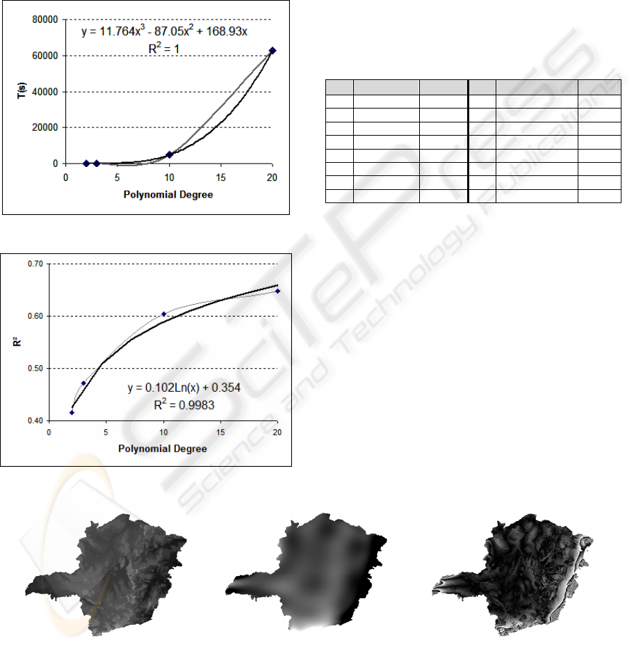
With the values from Table 2 and by using
polynomial regression, we get Equation 16 and
Equation 17 that estimate the time t(s) and R
2
,
respectively, with r = s.
sssst 93.16805.87764.11)(
23
+−=
,
R
2
= 1.0
(16)
354.0)ln(102.0)(
2
+= ssR
,R
2
= 0.9983
(17)
Figure 3: Processing time estimative.
Figure 4: Estimated error.
From Equation 16 and Equation 17 we simulated
the time processing in second t(s), and the
coefficient of regression R
2
, to adjusted a
polynomial to represent the landform attributes for r
= s, varying from 30 to 500 degree, as shown on
Table 3. As an example, for r = s = 500, using the
PC machine previously described, the polynomial
representing the state of Minas Gerais, will be
adjusted with R
2
=0.988 and will need 45.9 years to
generate the coefficients.
Table 3: Processing time in seconds t(s) and R
2
for the
polynomial of degree r in x and s in y, r = s, from 30 to
500 degrees.
r=s t(s) R
2
r=s t(s) R
2
30 244,351 0.70102 225 129,630,416 0.9065
40 620,373 0.73037 250 178,414,108 0.9173
60 2,237,780 0.77172 300 309,844,179 0.9359
80 5,479,562 0.80107 350 493,777,001 0.9516
90 7,886,055 0.81308 375 608,189,130 0.9587
100 10,910,393 0.82383 400 739,035,572 0.9652
150 37,770,215 0.86518 450 1,054,442,894 0.9772
200 90,663,786 0.89453 500 1,448,821,965 0.988
Using the DEM data source, an elevation map
was generated in gray tones, Figure 5-a, where can
be observed that the state of Minas Gerais has a
heavily uneven topography. With the coefficients of
the adjusted polynomial of degrees r = s = 20, the
elevation map was also generated, Figure 5-b. In
Figure 5-c, we show the relative errors computed
using the source data (DEM) and the estimated data
(polynomial).
Since we used only points that represent the
landform attributes of the state of Minas Gerais, the
bordering areas suffered heavy alterations,
generating non existent elevations. This anomaly can
be corrected by taking points that cross the limits of
the real area, for estimation of the polynomial
parameters.
Figure 5: Elevation map of Minas Gerais state generated by: (a) DEM of GTOPO project, (b) estimated polynomial with r =
s = 20 that represents the DEM and (c) the relative errors form the data source and the estimated data.
(a) (b) (c)
WEBIST 2008 - International Conference on Web Information Systems and Technologies
188

The elevations of DEM and the elevations
estimated by the polynomial of degrees r = s = 20
are displayed in classes in Table 4. By analysis of
those data we may verify that the classes are
comparable, although the adjusted polynomial
generates some values above the maximum and
below the minimum real elevations. It is believed
that with larger r and s, we can get better values of
R
2
and that will improve the accuracy of the
polynomial parameters.
4 CONCLUSIONS
Table 4: Elevation classes from the DEM source and
estimated polynomial for r = s = 20.
Elevation
Classes(m)
Points from
DEM (source
data)
Points from
estimated
polynomial
0 - 200 5,055 78,725
0201 - 400 48,866 42,757
0401 - 600 127,776 119,401
0601 - 800 249,762 222,355
0801 - 1000 226,481 158,256
1001 – 1200 51,055 47,817
1201 – 1400 22,334 16,348
1401 – 1600 4,482 9,823
1601 – 1800 811 6,443
1801 -2000 331 4,687
2001 – 2200 99 3,548
2201 – 2400 24 2,683
> 2400 27 9,451
Minimum Elevation 1 -4,374
Maximum Elevation 2,863 5,606
The adjusted polynomial of degree 20 in x and y has
441 coefficients. If we use the type float to store
them, it will be necessary 1,764 KB of storage. The
DEM, on the other hand, with 722,294 points,
requires at least 2 bytes to indicate the elevation of
each point, being necessary the total of 1,444 MB to
store it. The adjusted polynomial needs about
0.1221% of space used by the DEM. From the
results, it is verified that is possible to represent,
satisfactorily, the landform attributes of an area by a
high degree polynomial and the representation has
the advantage of smaller space. Additionally, the
functional representation of the landform attributes
allows larger efficiency, in time and space when
sending this information through networks.
Efficiency in time is real since, instead of sending an
image with millions of points, the coefficients of a
mathematical function are sent. Efficiency in space
is also obtained since, instead of storing the DEM,
we may store the coefficients that represent it. In this
methodology, larger polynomial degree, better is the
solution. For this work, a polynomial of degree 20
was used, however with a polynomial of degree 200
or larger, the results, statistically, would be better.
The presented methodology also has the advantage
of being easily adaptable for distributed processing.
REFERENCES
Burrough, P. A., 1986. Principles of Geographical
Information Systems for Land Resources Assessment.
Clarendon Press, Oxford, England.
Ervin, S. M., Hasbrouck, H. H., 2001. Landscape
Modeling: Digital Techniques for Landscape
Visualization. McGraw-Hill Professional Publishing.
Fowler, D., 2005. A Supercomputer in Every Home?.
NetNews.
INPE, 2001. Introdução à Ciência da GeoInformação.
INPE. São José dos Campos, SP, Brazil.
Noble, B., Daniel, J. W., 1986. Álgebra Linear Aplicada.
Prentice/Hall do Brasil, Rio de Janeiro, Brazil.
Seber, G. A. F., Wild C. J., 2005. Nonlinear Regression
John Wiley, New York, N.Y IEEE.
Tanenbaum, A. S., 2002. Computer Networks. 4th Edition,
Prentice Hall, Upper Saddle River, N.J..
U.S. Geological Survey GTOPO30, 2006. [Internet].
Available from: http://edc.usgs.gov/products/
elevation/gtopo30/gtopo30.html.
Zakon, R. H., 2006. Hobbes' Internet Timeline. [Internet].
Available from: http://www.zakon.org/robert/internet/
timeline/#Growth.
A MATHEMATICAL FORMULATION OF A MODEL FOR LANDFORM ATTRIBUTES REPRESENTATION FOR
APPLICATION IN DISTRIBUTED SYSTEMS
189
