INFORMATION SYSTEM PROCESS INNOVATION

EVOLUTION PATHS

Erja Mustonen-Ollila

Lappeenranta University of Technology, Department of Information Technology, P.O. Box 20

FI-53851 LAPPEENRANTA, Finland

Jukka Heikkonen

Helsinki University of Technology, Department of Biomedical Engineering and Computational Science (BECS)

P.O. Box 9203, FI-02015 TKK, Finland

Keywords: Empirical research, Longitudinal study, Case Study, IS process innovations, Evolution paths.

Abstract: This study identifies Information System process innovations’ (ISPIs) evolution paths in three organisations

using a sample of 213 ISPI development decisions over a period that spanned four decades: early

computing (1954-1965); main frame era (1965-1983); office computing era (1983-1991), and distributed

applications era (1991-1997). These follow roughly Friedman’s and Cornford’s categorisation of IS

development eras. Four categories of ISPI’s are distinguished: base line technologies, development tools,

description methods, and managerial process innovations. Inside the ISPI categories ISPI evolution paths

are based on the predecessor and successor relationships of the ISPIs over time. We analyse for each era the

changes and the dependencies between the evolution paths over time. The discovered dependencies were

important in understanding that the changes on ISPIs are developed through many stages of evolution over

time. It was discovered that the dependencies between the evolution paths varied significantly according to

the three organisations, the four ISPI categories, and the four IS development eras.

1 INTRODUCTION

We shall define IS process innovation (ISPI) as any

new way of developing, implementing, and

maintaining information systems in an

organisational context (Swanson, 1994). In

Swanson’s (1994) terminology, ISPIs cover both

technological (Type Ia, tool innovations (TO) and

core technology innovations (T)) as well as

administrative innovations (Type Ib, management

innovations (M) and description innovations (D). In

addition to above concepts an important concept

defined is development units. Development units are

generally: “regions involved as part of the setting of

interaction, having definite boundaries, which help

to concentrate interaction in one way or another”

(Giddens, 1984, p. 375). We denote development

units as locales.

One aspect in ISPI evolution is the dynamics in

the development practices, i.e. how the set of ISPIs

used changes over time in locales (Friedman and

Cornford, 1989). Based on Friedman and Cornford

(1989) we classify ISPIs into several eras. We will

recognise accordingly four ISPI generations. The

first generation (from the late 1940s until the mid

1960s) is largely hampered by “hardware

constraints”, i.e. hardware costs and limitations in its

capacity and reliability. The second generation

(from the mid 1960s until the early 1980s), in turn,

is characterised by “software constraints”, i.e. poor

productivity of systems developers and difficulties

of delivering reliable systems on time and within

budget. The third generation (early 1980s to the

beginning of 1990s), was instead driven by the

challenge to overcome “user relationships

constraints”, i.e. system quality problems arising

from inadequate perception of user demand and

resulting inadequate service. Finally, the fourth

generation (from the beginning of 1990s) was

affected by “organisational constraints”. In the latter

case the constraints arise from complex interactions

171

Mustonen-Ollila E. and Heikkonen J. (2008).

INFORMATION SYSTEM PROCESS INNOVATION EVOLUTION PATHS.

In Proceedings of the Tenth International Conference on Enterprise Information Systems - ISAS, pages 171-178

DOI: 10.5220/0001667401710178

 SciTePress

between computing systems and specific

organisational agents including customers and

clients, suppliers, competitors, co-operators,

representatives and public bodies (Friedman and

Cornford, 1989). In this study time generation one is

1954-1965; generation two is 1965-1983; generation

three is 1983-1991; and generation four is 1991-

1997.

After Tolvanen (1998) ISPI evolution is defined

as how the general requirements are adapted into the

ISD situation in hand. ISPI subcategories inside the

four ISPI categories are denoted as ISPI evolution

paths, and they are based on the predecessor and

successor relationships of the ISPIs over time

(Smolander et al., 1989). The relationship means

that an ISPI is based more or less on the previously

existing and used ISPI. The successor of an ISPI

follows after the ISPI predecessor on time.

2 FIELD STUDY ON ISPI

EVOLUTION PATHS

In our longitudinal study three Finnish organisations

were used as case examples over a 43-year time

period. Our investigation is crucial for ascertaining

how the ISPI evolution paths were changed and

were dependent from each other involving a

longitudinal perspective with several organisational

environments. For studying how the dependencies

of the ISPI evolution paths inside the four ISPI

categories changed over time Table 1 was created

from the data.

We chose a qualitative case study (Laudon,

1989; Johnson, 1975; Curtis et al., 1988) with a

multi-site study approach, where we investigated

three organisational environments, known here as

companies A, B, and C. Our study forms a

descriptive case study (Yin, 1993): it embodies time,

history and context, and it can be accordingly

described as a longitudinal case study, which

involves multiple time points (Pettigrew, 1985,

1989, 1990). Research approach followed

Friedman’s and Cornford’s (1989) study, which

involved several generations and time points.

Because the bulk of the gathered data was

qualitative, consisting of interviews and archival

material, we adopted largely historical research

methods (Copeland and McKenney, 1988; Mason et

al., 1997a, 1997b). Our definitions of ISPI evolution

paths for ISPI development decisions formed the

basis for interviews and collection of archival

material. Empirical data contained tape-recorded

semi-structured interviews dealing with the

experiences from developing and using ISPIs, and

archival files and collected system handbooks,

system documentation and minutes of meetings

(Järvenpää, 1991). We thus used triangulation to

verify veracity of data by using multiple data

sources, and arranged the obtained data is a

manuscript.

Using the validated information retrieved from

the manuscript, a table was organized for each

incidence of an ISPI: a description of the company,

the year when the development decision was made;

Table 1: ISPI evolution paths.

ISPI categories (D, M, TO, T) ISPI subcategories inside the ISPI categories: evolution paths EVO1 to EVO4

Description methods (D) EVO1: Wall technique/wall picture and entity analysis

EVO2: Methods for strategic development (function processes, re-engineering)

denoted as process modelling approaches

EVO3: Design methods and techniques, such as Object Modelling Technique

(OMT), Object Orientation (OO) etc.

Project management and control

procedures (M)

EVO1: Phase models

EVO2: Project instructions and management

EVO3: Standards and instructions

Development tools (TO) EVO1: CARELIA, Visual Basic (VB), CAREL etc.

EVO2: Application Development Workbench (ADW) , S-Designer, Power-Designer

EVO3: Data communication tools

EVO4: Database handling tools and databases

Technology innovations (T) EVO1: Programming languages

EVO2: Query languages

EVO3: Modular computing: programming procedures, and techniques

EVO4: Operating environment tools (different tools for different environments)

ICEIS 2008 - International Conference on Enterprise Information Systems

172

the IS project; the locale; an incidence of the

evolution path in each of the development was

made; the IS project; the locale; an incidence of the

evolution path in each of the development decisions.

Thus, we found 213 development decisions where

they were present. Then the data set was converted

into a data matrix based on the presence of a specific

feature. For a single development decision, called s

sample the maximum number of ISPI evolution

paths was four. The data consisted of 26 binary

variables: 14 variables for ISPI evolution paths

(“wall technique/wall picture and entity analysis” to

“operating environment tools (different tools for

different environments”), three variables for three

locales, three variables for four time generations,

four variables for the four ISPI categories, and one

variable for internally or externally developed

ISPIS. The presence of feature was denoted by 1 and

absence by 0 (like c.f. Ein-Dor and Segev, 1993).

(ISPI time generation one was left out due to lack of

data).

From these 26 variables 14 were selected as

independent variables which were used to explain

the rest of the 12 dependent variables. The

independent variables were (1) Description methods

EVO1: wall technique/wall picture and entity

analysis, (2) Description methods EVO2: methods

for strategic development, denoted as process

modelling approaches, (3) Description methods

EVO3: design methods and techniques, such as

OMT, OO etc., (4) Project management and control

procedures EVO1: phase models, (5) Project

management and control procedures EVO2: project

instructions and management, (6) Project

management and control procedures EVO3:

standards and instructions, (7) Development tools

EVO1: Carelia, Visual Basic, Carel etc, (8)

Development tools EVO2: ADW, S-designer,

power-designer, (9) Development tools EVO3: data

communications tools, (10) Development tools

EVO4: database handling tools and databases, (11)

Technology innovations EVO1: programming

languages, (12) Technology innovations EVO2:

query languages, (13) Technology innovations

EVO3: modular computing (programming

procedures and techniques), and (14) ISPI

Technology innovations EVO4: operating

environment tools. The reason for this selection of

the independent and dependent variables was based

on our research question.

The variation in the dependencies in the ISPI

evolution paths was modelled with the component

plane and the U-matrix (unified distance matrix)

representations of the Self-Organizing Map (SOM)

(Kohonen, 1989, 1995; Ultsch and Siemon, 1990).

The SOM is a vector quantisation method to map

patterns from an input space V

onto typically lower

dimensional space V

of the map such that the

topological relationships between the inputs are

preserved. This means that the inputs, which are

close to each other in input space, tend to be

represented by units (codebooks) close to each other

on the map space which typically is a one or two

dimensional discrete lattice of the codebooks. The

codebooks consist of the weight vectors with the

same dimensionality as the input vectors. The

training of the SOM is based on unsupervised

learning, meaning that the learning set does not

contain any information about the desired output for

the given input, instead the learning scheme try to

capture emergent collective properties and

regularities in the learning set. This makes the SOM

especially suitable for our type of data where the

main characteristics emerging from the data are of

interest, and the topology-preserving tendency of the

map allows easy visualisation and analysis of the

data.

Training of the SOM can be either iterative or

batch based. In the iterative approach a sample,

input vector x(n) at step n, from the input space V

, is

picked and compared against the weight vector w

codebook with index i in the map V

. The best

matching unit b (bmu) for the input pattern x(n) is

selected using some metric based criterion, such as

⎪⎪x(n)-w

⎪⎪ = min

⎪⎪ x(n)-w

⎪⎪, where the parallel

vertical bars denote the Euclidean vector norm. The

weights of the best matching and the units in its

topologic neighbourhood are then updated towards

x(n) with rule w

(n+1) = w

(n) +

(n) h

i,b

(n) (x(n)

– w

(n)), where i

∈

and 0

≤α

(n)

≤

1 is a scalar

valued adaptation gain. The neighbourhood function

i,b

(n) gives the excitation of unit i when the best

matching unit is b. A typical choice for h

i,b

(n) is a

Gaussian function. In batch training the gradient is

computed for the entire input set and the map is

updated toward the estimated optimum for the set.

Unlike with the iterative training scheme the map

can reach an equilibrium state where all units are

exactly at the centroids of their regions of activity

(Kohonen, 1995). In practice batch training can be

realised with a two step iteration process. First, each

input sample is assigned best matching unit. Second,

the weights are updated with

∑

i,b(x)

x /

∑

i,b(x)

. When using batch training

usually little iteration over the training set are

sufficient for convergence. In our experiences we

INFORMATION SYSTEM PROCESS INNOVATION EVOLUTION PATHS

173

used batch learning scheme.

According to the experiences it is desirable to

divide the training into two phases: 1) initial

formation of a coarsely correct map, and 2) final

convergence of the map. During the first phase the

width of the function h

i,b(x)

should be large as well as

the value of

should be high. The purpose of the

first stage is to ensure that a map with no

``topological defects'' is formed. During learning

these two parameters should gradually decrease

allowing finer details to be expressed in the map.

However, in most cases these choices are not so

crucial, because the method tends to perform well

for a wide range of parameter settings.

The mathematical properties of the SOM

algorithm have been considered by several authors

(e.g. Kohonen, 1989, 1995; Luttrell, 1989; Cottrel,

1998). Briefly, it has been shown that after learning

the weight vectors in the map with no “topological

defects” specify the centers of the clusters covering

the input space and the point density function of

these centers tends to approximate closely the

probability density function of the input space. Such

mapping, of course, is not necessarily unique.

The basic SOM based data analysis procedure

typically involves training a 2-D SOM with the

given data, and after training, various graphs are

plotted and qualitatively or even quantitatively

analysed by experts. The results naturally depend on

the data, but in the cases, where there are clear

similarities and regularities in the data, these can be

observed by the formed pronounced clusters on the

map. These observable clusters can provide clues to

the experts on the dependencies and characteristics

of the data, and some data clusters of particular

interest can be picked for further more detailed

analysis. To help this type of exploratory analysis, a

typical visualisation step is so called component

plane plotting (Kohonen, 1995), where the

components of codebook vectors are drawn in the

shape of the map lattice. By looking component

planes of two or more codebook variables it is

possible to observe the dependencies between the

variables. The above type of component plane

analysis was performed on the data analysed here.

The U-matrix (unified distance matrix)

representation of the SOM (Ultsch and Siemon,

1990) visualises the distances between the neurons,

i.e. codebooks. The distance between the adjacent

neurons is calculated and presented with different

colours. If a black to white colouring schema is used

typically a dark colour between the neurons

corresponds to a large distance and thus a gap

between the codebooks in the input space. A dark

colouring between the neurons signifies that the

codebook vectors are close to each other in the input

space. Dark areas can be thought of as clusters and

light areas as cluster separators. In our case we used

blue to red colouring schema for better visualization

properties; blue colour corresponds to a shorter

distance and red to a larger one whereas yellow

colour between those as shown by colour bar in each

U-matrix figure. This U-matrix representation can

be a helpful when one tries to find clusters in the

input data without having any prior information

about the clusters. Of course, U-matrix does not

provide definite answers about the clusters, but it

gives clues regarding what similarities (clusters)

there may be in the data by revealing possible

cluster boundaries on the map. Teaching SOM and

representing it with the U-matrix offers a fast way to

get insight on the data distribution. A simple

algorithm for a U-matrix is as follows. For each

node in the map, compute the average of the

distances between its weight vector and those of its

immediate neighbours. The average distance is a

measure of a node's similarity between it and its

neighbours.

The SOM map was trained with the data

consisting of 213 samples were each sample

consisted of 14 independent variables (i.e. input

space dimensionality is 14). After training, the dark

units (the low values of the U-matrix) of the SOM

represent the clusters, and light units (the high

values of the U-matrix) represent the cluster borders.

3 RESEARCH FINDINGS AND

ANALYSIS

Our main research problem was to investigate “How

have the dependencies in the evolution paths inside

the ISPI categories changed over time?” The U-

matrix visualises the distances between

neighbouring map units, and helps to see the cluster

structure of the map. The high values of the U-

matrix (light units) indicate a cluster border. The

elements of the same clusters are indicated by

uniform areas of low values (dark units) and thus

similar data is grouped together. The colour bar

indicates the colour and its meaning.

Figures 1-4 present the component planes and

the U-matrices of the SOMs of 4x6 units for the

ISPI categories M (project management and control

procedures), T (technology innovations), TO

(development tools), and D (description methods)

ICEIS 2008 - International Conference on Enterprise Information Systems

174

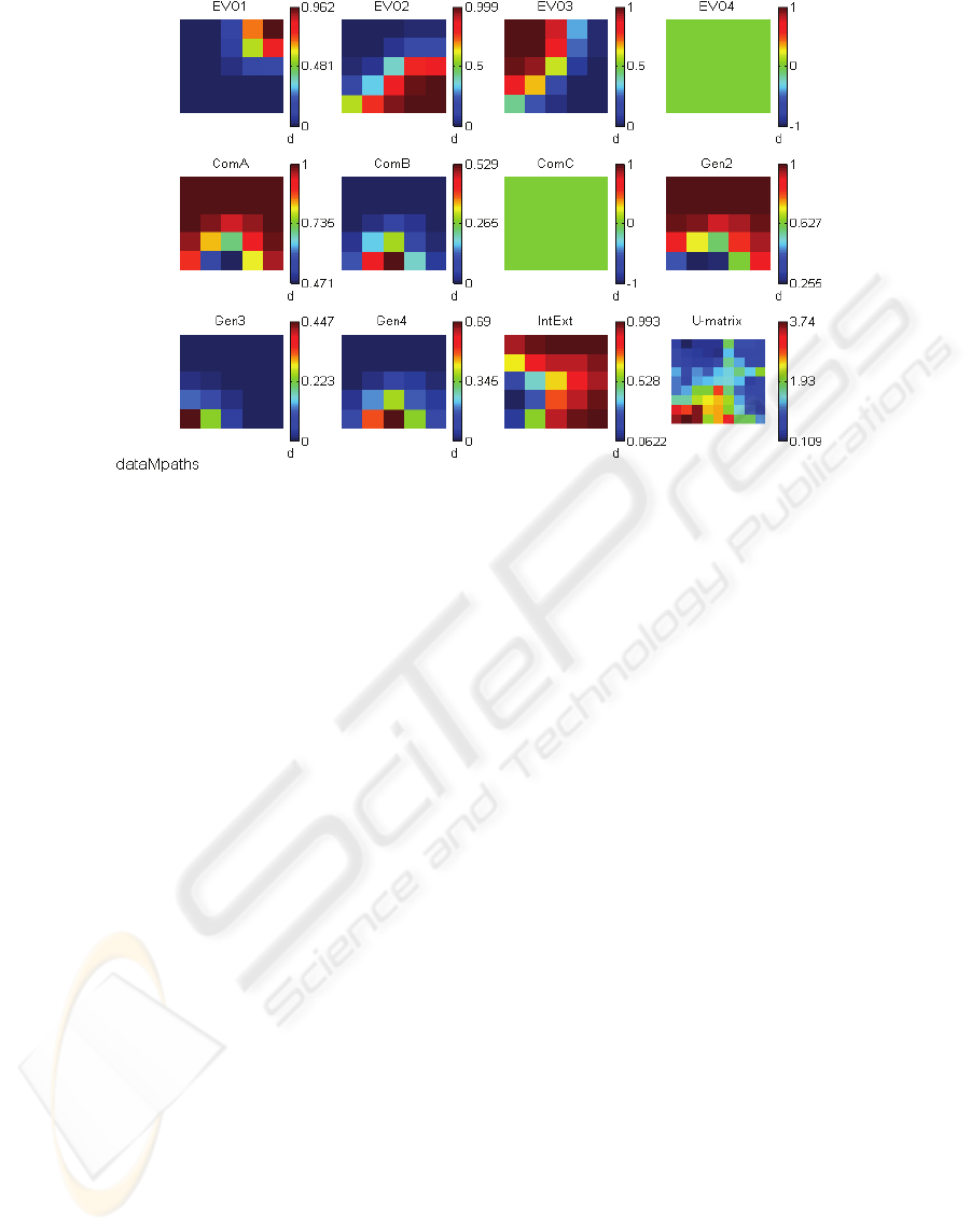
Figure 1: The component planes and the U-matrix in a SOM of 4x6 units in the ISPI category M.

respectively. ComA, ComB, and ComC are denoted

as Company A, B, and C respectively. Time

generation two, three, and four are denoted as Gen2,

Gen3, and Gen4 respectively. The variable IntExt

seen on the component plane figures shows if the

value of the variable is 1 (Int) or 0 (Ext), and thus

Int and Ext variables are complements to each other

The light green colour in a component plane

variable, such as in “EVO4 and ComC”, is constant

being 1 or 0, and it has no variation on the data. The

blue units (the low values of the U-matrix) of the

SOM represent the clusters, and the red units (the

high values of the U-matrix) represent the cluster

borders in the colour bar. Therefore the colour bars

show the values of the variables.

The data for time generation two was separated

from that of time generations three and four due to

our research question. Time generation one was left

out due to the lack of data.

From the U-matrix in Figure 1 one can clearly

see three clusters. The first cluster is situated in the

upper left corner of the U-matrix. The second cluster

is situated in the upper right corner of the U-matrix,

and the third cluster is situated in the lower right

corner of the U-matrix (blue color) for the ISPI

category M.

By looking at the variable values in these three

clusters, we observe the following dependencies

between the variables. In the first cluster, high

values exists in the variables EVO3 (standards and

instructions), ComA, and Gen2. In the second

cluster, high values exists in the variables EVO3

(standards and instructions), ComA and Gen2. In the

third cluster, high values exists in the variables

EVO2 (project instructions and management),

ComA, and Gen2. Thus, EVO3 (standards and

instructions) and EVO2 (project instructions and

management) were dependent on company A, and

time generation two in ISPI category M.

After investigating the U-matrix in the Figure 2

we discovered two clusters. The first cluster is in the

upper part of the U-matrix, and the second cluster is

in the lower part of the U-matrix (blue color).

Between these two clusters there is the cluster

border (red and yellow color).

By looking at the variable values in these two

clusters, we observe the following dependencies

between the variables. In the first cluster, high

values existed in the variables EVO4 (operating

environment tools), ComB, ComC, Gen3, and Gen4.

In the second cluster, high values existed in the

variables EVO1 (programming languages), EVO2

(query languages), EVO3 (modular computing),

ComA and Gen2.

Therefore, EVO1, EVO2, and EVO3 were

dependent on company A in the second time

generation in ISPI category T. EVO4 was dependent

both on company B in the time generation three, and

company C in the time generation four in ISPI

category T.

INFORMATION SYSTEM PROCESS INNOVATION EVOLUTION PATHS

175

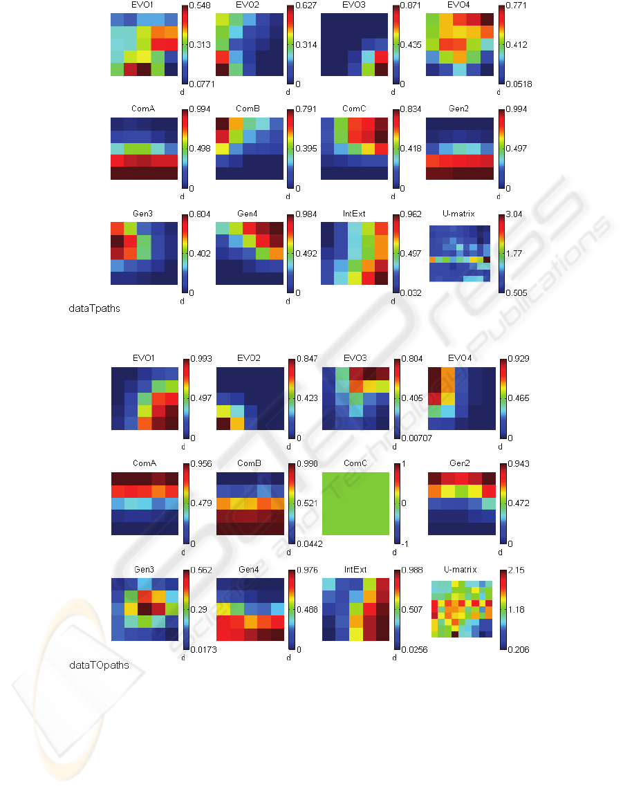
Figure 2: The component planes and the U-matrix in a SOM of 4x6 units in the ISPI category T.

Figure 3: The component planes and the U-matrix in a SOM of 4x6 units in the ISPI category TO.

After studying the U-matrix in the Figure 3 we

noticed only one cluster in the lower part of the U-

matrix (blue color). By looking at the variable value

in this single cluster, we observe that the following

dependencies between the variables existed: high

values existed in the variables EVO1 (Carelia,

Visual Basic, Carel etc.), ComB, and Gen4.

Thus, EVO1 was dependent on company B in

the fourth time generation in ISPI category TO.

In the Figure 4, the component planes (the

variables EVO1 to IntExt), and the U-matrix were

investigated and the three clusters are discovered.

The first cluster is in the upper left part of the U-

matrix, the second cluster is in the upper right part

of the U-matrix (blue color), and the third cluster is

in the lower right part of the U-matrix. Between

these three clusters there is the cluster border (red

and yellow color).

ICEIS 2008 - International Conference on Enterprise Information Systems

176

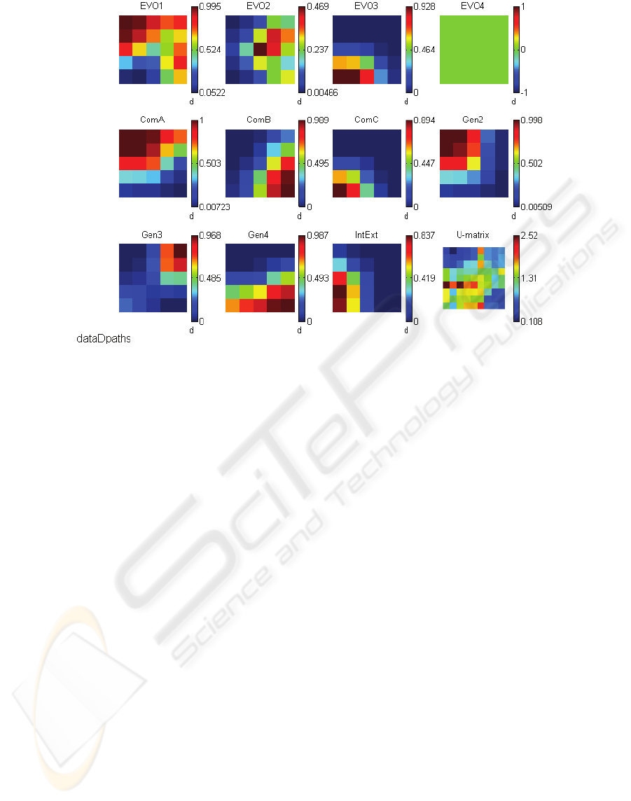
Figure 4: The component planes and the U-matrix in a SOM of 4x6 units in the ISPI category D.

By looking at the variable values in these three

clusters, we observe the following dependencies

between the variables. In the first cluster, high

values existed in the variables EVO1 (wall

technique/wall picture and entity analysis), ComA,

and Gen2. In the second cluster, high values existed

in the variables EVO2 (methods for strategic

development), ComA, and Gen2. In the third cluster,

high values existed in the variables EVO1, ComB,

and Gen4. Thus, EVO1, and EVO2 were dependent

on company A in the second time generation. EVO1

was dependent on company B in the fourth time

generation in ISPI category D.

4 DISCUSSION AND

CONCLUSIONS

Based on found clusters in the Figures 1, 2, 3, and 4

we discovered that the dependencies between the

evolution paths varied significantly according to the

companies A, B, and C, the four ISPI categories (M,

T, TO, and D), and the four time generations. Even

if we did not measure a correlation or a linear

relationship between the evolution paths, the

dependencies were discovered.

Our field study over time indicated that

evolution paths varied according to the time

generations and locales. Before the outsourcing in

1984 evolution paths were discovered from the

management and control procedures category,

technology innovation category, and description

methods category ISPIs. After outsourcing no

evolution paths were found in management control

procedures ISPIs, and companies B and C began to

concentrate on development tools, and technology

innovations. Therefore when comparing the

evolution paths in company A and B and C it was

discovered, that no evolution paths existed in

managerial control procedures and description

methods ISPI categories after the outsourcing. The

findings indicated that company B and C shifted

their interest to technology innovations and

development tools.

The present study has implications to the

practitioners, research, and methodology. An

important implication to methodology is the use of

multi method research approach. Even if our case

study has weaknesses, we produced a logical chain

of evidence with multiple data points. Using U-

matrix representation as the analysing tools was

proved to be suitable to the data analysis, even if

there is no study were such a method is previously

applied. Empirical research on how ISPI evolution

paths are changed and are dependent from each

other involving a longitudinal perspective with

several organisational environments and time

generations is lacking. ISPI evolution literature is

very rare. This longitudinal data is important,

INFORMATION SYSTEM PROCESS INNOVATION EVOLUTION PATHS

177

because a horizontal survey research would not have

given answers to our research question how ISPI

evolution paths were changed over time.

REFERENCES

Copeland, D.G., McKenney, J.L., 1988. Airline

Reservations Systems: Lessons from History, MISQ,

pp. 353-370.

Curtis, B., Krasner, H., Iscoe, N., 1988. A Field Study of

the software design process for large systems,

Communications of the ACM, Vol. 31, No. 11, pp.

1268-1287.

Ein-Dor, P., Segev, E., 1993. A Classification of

Information Systems: Analysis and Interpretation,

Information Systems Research, Vol. 4, No. 2, pp. 166-

204.

Friedman, A., Cornford D., 1989. Computer Systems

Development: History, Organization and

Implementation, John Wiley & sons.

Giddens, A., 1984. The Constitution of Society, Polity

Press.

Johnson, J. M., 1975. Doing field research, The Free

Press.

Järvenpää, S., 1991. Panning for Gold in Information

Systems Research: ‘Second-hand’ data”, Proceedings

of the IFIP TC/WG 8.2, Copenhagen, Denmark, 14-16

December, pp. 63-80.

Kohonen, T., 1989. Self-Organization and Associative

Memory, Springer-Verlag, Berlin, Heidelberg.

Kohonen, T., 1995. Self-Organized Maps. Berlin:

Springer-Verlag.

Laudon, K. C., 1989. Design Guidelines for Choices

Involving Time in Qualitative Research, Harward

Business School Research Colloquium, The

Information Systems Research Challenger: Qualitative

Research Methods, Vol. 1, pp. 1-12.

Luttrell, S. P., 1989. Self-Organization: A derivation from

first principles of a class of learning algorithms.

Proceedings of the IJCNN’89 International Joint

Conference On Neural Networks, Vol. 2, pp. 495–498.

Mason, R.O., McKinney, J.L., Copeland, D.C., 1997a.

Developing an Historical Tradition in MIS Research,

MISQ, Vol. 21, No. 3, pp. 257-278.

Mason, R.O., McKenney, J.L., Copeland, D.G., 1997b. A

Historical Method for MIS Research: Steps and

Assumptions, MISQ, Vol. 21, No. 3, pp. 307-320.

Pettigrew, A., 1985. The Wakening Giant, Continuity and

Change in ICI.

Pettigrew, A., 1989. Issues of Time and Site Selection in

Longitudinal Research on Change, Harward Business

School Research Colloquium, The Information

Systems Research Challenger: Qualitative Research

Methods, Vol. 1, pp. 13-19.

Pettigrew A.M., 1990. Longitudinal field research on

change: theory and practice, Organization Science,

Volume 1, No. 3, pp. 267-292.

Smolander, K., Lyytinen, K., Tahvanainen, V-P., 1989.

Family tree of methods (in Finnish), Syti-project,

(internal paper), University of Jyväskylä, Finland.

Swanson, E. B., 1994. Information Systems Innovation

Among Organizations, Management Science, Vol. 40,

No. 9, pp. 1069-1088.

Tolvanen, J-P., 1998. Incremental Method Engineering

with Modeling Tools: Theoretical Principles and

Empirical Evidence, Dissertation thesis, University of

Jyväskylä.

Ultsch, A., Siemon, H.P., 1990. Kohonen's self organizing

feature maps for exploratory data analysis. In

Proceeding of INNC'90, International Neural Network

Conference, pp. 305-308, Dordrecht, Netherlands,

Kluwer.

Yin, R.Y., 1993. Applications of Case Study Research,

Applied Social Research Methods series, Vol. 34,

SAGE publications.

ICEIS 2008 - International Conference on Enterprise Information Systems

178