
DEFINING THE IMPLEMENTATION ORDER OF SOFTWARE
PROJECTS IN UNCERTAIN ENVIRONMENTS
Eber Assis Schmitz, Antonio Juarez Alencar, Marcelo C. Fernandes and Carlos Mendes de Azevedo
Institute of Mathematics and Electronic Computer Center, Federal University of Rio de Janeiro, Rio de Janeiro - RJ, Brazil
Keywords:
Minimum Marketable Feature, Incremental Funding Method, Project Management and Business Performance.
Abstract:
In the competitive world in which we live, where every business opportunity not taken is an opportunity handed
to competitors, software developers have distanced themselves, in both language and values, from those who
define the requirements that software has to satisfy and come up with the money that funds its development
process. Such a distance helps to reduce or, in some cases, completely eliminate the competitive advantage that
software development may provide to an organization; transforming this value creation activity into a business
cost that is better kept low and under tight control. This article proposes a method for obtaining the optimal
implementation order of software units in an information technology development project. This method,
which uses a combination of heuristic procedures and Monte Carlo simulation, takes into consideration the
fact that software development is generally carried out under cost and investment constraints in an uncertain
environment, whose proper analysis indicate how to obtain the best possible return on investment. The article
shows that decisions made under uncertainty may be substantially different from those made in a risk-free
environment.
1 INTRODUCTION
In the last decades Information Technology (IT) has
become an important component of business strategy.
Therefore, it should come as no surprise that in the
American service industry alone IT is responsible for
more than half of capital investment. In this day and
age, IT has become the informational infra-structure
of many organizations, helping the generation of new
services and products, the creation of innovativeman-
agerial structures, to access new markets and establish
new forms of speeding up the delivery of services and
goods (Scott, 2006).
However, in the course of time, the practice of
software development has become increasingly dis-
connected from those who define the requirements
that software have to satisfy and fund the software
development process. While IT professionals are gen-
erally concerned with software development method-
ologies, its related supporting tools, classes of objects
and use cases, business oriented personnel are preoc-
cupied with product marketable features, project cash
flows, competitive advantage and, ultimately, return
on investment (Denne and Cleland-Huang, 2003).
This should come as no surprise as business related
subjects are seldom part of the regular computer
science or computer engineering curriculum at both
undergraduate and graduate level (Joint Task Force,
2005; Verhoef, 2005).
This disconnection, in both language and value,
has two important consequences for software devel-
opment. First, as IT professionals become more tech-
nical and less business oriented, software develop-
ment tends to be perceived by high management as
a business cost, that is better kept low and under tight
control. Second, the acceptable payback time of IT
projects is likley to become much shorter, making
it very difficult to develop long term projects, even
though they might be strategically relevant. All of
this, obviously, affects the way IT is used in the strate-
gic context, transforming, in many circumstances, a
value creation activity such as software development
in a mere outsourceable part of business (Denne and
Cleland-Huang, 2003).
23
Assis Schmitz E., Juarez Alencar A., C. Fernandes M. and Mendes de Azevedo C. (2008).
DEFINING THE IMPLEMENTATION ORDER OF SOFTWARE PROJECTS IN UNCERTAIN ENVIRONMENTS.
In Proceedings of the Tenth International Conference on Enterprise Information Systems - ISAS, pages 23-29
DOI: 10.5220/0001670200230029
Copyright
c
SciTePress

Although, it is generally accepted that software
development should be managed interactively as a re-
sult of smaller functional ready-to-use parts, little at-
tention has been given on how software development
should be funded. While agile methods such as Scrum
and Extreme Programming (XP), do favor the con-
struction of such parts, the full value that the right
combination of these parts brings to business are still
not fully unleashed (Germain and Robillard, 2005).
This article proposes a method for identifying the
optimum implementation order of software units in
an IT project. Such an order helps to place software
at the center of business strategic decisions, mak-
ing it possible to develop complex information sys-
tems from a relatively small investment. The method,
based upon a combination of heuristic procedures and
Monte Carlo simulation, takes into account that soft-
ware development takes place in an uncertain envi-
ronment, being subjected to cost and risk constraints.
2 CONCEPTUAL FRAMEWORK
Typically, the buying process of any product by con-
sumers has four main components: (1) there is a need
that has to be satisfied, (2) there is at least one product
that is perceived as satisfying that need, (3) there is
money available to pay for the product, and (4) con-
sumers are willing to pay what they have asked for
(Kotler and Armstrong, 2007). While simple prod-
ucts have a reduced set of features for which people
are willing to pay, software may have a large collec-
tion of such features (Little, 2004).
According to Denne and Cleland-Huang (Denne
and Cleland-Huang, 2003; Denne and Cleland-
Huang, 2004; Cleland-Huang and Denne, 2005) soft-
ware minimum marketable features, or MMFs for
short, are software units that have an intrinsic mar-
ketable value. These software units create market
value to business in one or several of the following
areas:
• Competitive differentiation - the software unit al-
lows the creation of service or product features
that are valued by customers and that are different
from anything else being offered in the market;
• Revenue generation - although the software unit
does not provide any unique valuable features to
customers, it does provide extra revenue by offer-
ing the same quality as other products in the mar-
ket for a better price;
• Cost savings - the MMF allows business to save
money by making one or more business processes
cheaper to run;
• Brand projection - by building the software unit
the business projects itself as being technologi-
cally advanced; and
• Enhanced customer loyalty - the software unit in-
fluences customers to buy more, more frequently
or both.
Moreover, the total value brought to a company
by a software consisting of several interdependent
MMFs, each one with its own cash flow stream and
precedence restrictions is highly dependent on the or-
der of implementation of the MMFs.
Although an MMF is a self-contained unit, it is
often the case that an MMF can only be developed
after other project parts have been completed. These
project parts may be either other MMFs or the archi-
tectural infrastructure, i.e. the set of basic features
that offers no direct value to customers, but that are
required by the MMFs.
The architecture itself can usually be decomposed
into self-contained deliverable elements. These el-
ements, called architectural elements, or AEs for
short, enables the architecture to be delivered accord-
ing to demand, further reducing the initial investment
needed to run a project. For instance, in a web-based
software system, the graphic interface library that al-
lows software units to share a common graphic iden-
tity is an architectural elements, as it has no value to
customers, but common sense indicate that no soft-
ware unit should be developed before it is built.
Figure 1 presents the precedence graph of a set
of MMFs from an example taken from Denne and
Cleland-Huang (Denne and Cleland-Huang, 2003).
Note that A, B, ···, D are software-building activi-
ties and that an arrow going from A to B, i.e. A → B,
indicate that the work on MMF A has to be completed
before the work on B can start.
A B C
D
E
Start Finish
Figure 1: The precedence graph of a set of MMFs.
Table 1 shows the net Cash-Flow Stream (CFS) in
US dollars of each MMF in Figure 1. For instance
consider MMF A. It requires an initial investment of
$50 thousand to be built. Once it is completed it gen-
erates a net revenue of $45 thousand per time period
for a total of eight periods. MMF E, on the other hand,
requires a higher investment of $60 thousand and gen-
erates a net revenue of $30 thousand per time period.
ICEIS 2008 - International Conference on Enterprise Information Systems
24
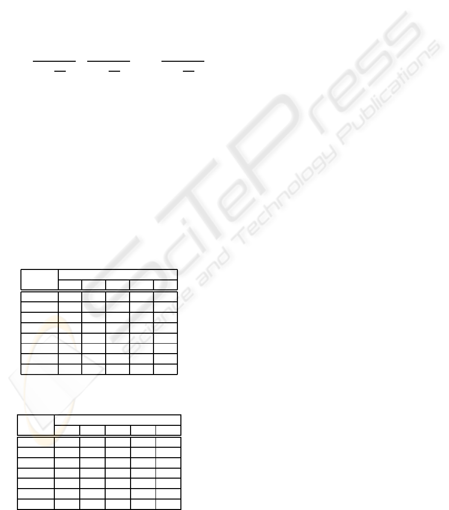
Because it is improper to perform mathematical
operations on monetary values without taking into ac-
count an interest rate, in order to compare the business
value of different MMFs one has to resort to their dis-
counted cash-flow. Table 2 shows the sum of the dis-
counted cash-flow of each MMFs in Figure 1, consid-
ering a discount rate of 2.4% per time period. Such a
sum is the the net present value (NPV) of all cash flow
elements of an MMF considering that its development
starts at period n ∈ [1..7]. For instance, according to
the information presented in Table 2, if MMF A is de-
veloped in the first period, it yields a net present value
(NPV) of $231 thousand, i.e.
NPV
A,1
=
−50
1+
2.4
100
1
+
45
1+
2.4
100
2
+···+
45
1+
2.4
100
8
= $231 thousand
If A is developed in the second period, it yields a
NPV
A,2
of $189, in the third $149 and so on.
Obviously, not all MMFs can be developed in the
first period. The precedence graph presented in Figure
1 indicates that only MMF A and D can be developed
at that time. Because in this example each MMF re-
quires exactly a period to be developed, MMF C can-
not be developed until the third period. Furthermore,
each particular sequence of MMF yields its own re-
turn on investment. For instance, sequence DABCE
yields an NPV of $799 thousand, i.e.
NPV(DABCE) = NPV
D,1
+ NPV
A,2
+ ·· · + NPV
E,5
Table 1: CFS of a set of MMFs in thousands of US dollars.
Period MMF
A B C D E
1 -50 -40 -20 -50 -60
2 45 60 35 50 30
3 45 60 35 50 30
4 45 60 35 50 30
5 45 60 35 50 30
6 45 60 35 50 30
7 45 60 35 50 30
8 45 60 35 50 30
Table 2: NPV of cash-flow streams starting at different pe-
riods.
Period MMF
A B C D E
1 231 334 198 262 128
2 189 278 165 216 101
3 149 223 133 170 74
4 109 169 102 126 48
5 70 117 71 83 23
6 32 66 41 40 -2
7 -5 16 12 -1 -26
= $262+ $189+ ···+ $23 = $799,
while sequence ABDCE yields $804 thousand.
MMF identification and ordering is possibly the
most important step in the software development pro-
cess in this day and age. The advantages of dividing
a software project into MMFs are numerous:
• Large and complex systems can be developed
with a relatively small investment,
• Return on investment in software development is
maximized, together with return on investment in
IT related areas and projects,
• Demand for shorter investment periods and pay-
back time is addressed,
• Faster time-to-market of software products and
also of products that depend upon software devel-
opment,
• Bring financial discipline into the software devel-
opment project, and
• Position the software development process as a
value creation activity in which business analysis
is an integral part of it.
Although dividing a software project into MMFs
and AEs is still an open problem, (Rashid et al., 2003)
have given the first steps in the right direction by sug-
gesting how software module and architectural ele-
ments may be derived from requirements.
In formal terms a network of MMFs is an
acyclic directed graph G = (V, E), where V =
{M
1
, M
2
, ··· , M
n
} is the ordered set of MMFs and
E = {(M
i
, M
j
)|1 ≤ i ≤ n and 1 ≤ j ≤ n} is the set of
edges, showing the development dependency relation
that hold among MMFs. For reasons of simplicity we
do not include the two dummy MMFs Start and Fin-
ish, which take no time to be completed and yield no
net present value, representing the start and finishing
point of the development of a software as a whole.
For a given total software life cycle T and a discount
interest rate α, each element M
i
∈ V is characterized
by the following parameters:
• CFS
i,t
– the value of cash flow element of M
i
at
period t, and
• NPV
i,t
– the present value of the cash-flow stream
of M
i
starting at a given time t, and
• D
i
– the number of time periods required to de-
velop M
i
,
where 1 ≤ t ≤ T and 1 ≤ D
i
≤ T.
A valid sequence VS is an ordered set of MMFs
satisfying the following restrictions
• All MMFs belong to the sequence and are listed
exactly once,
DEFINING THE IMPLEMENTATION ORDER OF SOFTWARE PROJECTS IN UNCERTAIN ENVIRONMENTS
25
• Only one MMF can be in the implementation pro-
cess at any given time period,
• The process of developing an MMF can only start
after its precedent MMFs are completed,
• The first MMF must start at time zero and
• Apart from the last, there is no time delay between
the end of one MMF and the start of the next one.
In our example, there are ten valid sequences:
ABCDE, ABDCE, ABDEC, ADBCE, ADBEC,
ADEBC, DEABC, DAEBC, DABEC and DABCE.
Given an MMF precedence graph, one is inter-
ested in finding a valid sequence v
1
·· ·v
n
, for v
1≤i≤n
∈
V, such that
NPV
v
1
,1
+
n
∑
i=2
NPV
v
i
,
∑
i−1
j=1
D
v
j
is maximized.
The problem of finding the valid sequence that de-
livers the maximum NPV was shown to be in the cat-
egory of NP-hard problems by Denne and Cleland-
Huang (Denne and Cleland-Huang, 2003), which also
showed several heuristics to find polynomial-time ap-
proximations to the optimal solution.
3 CASH-FLOW STREAM
PATTERNS
The estimated benefits generated by a software
project composed of several MMFs is most usually
expressed as a fixed net present value. See Table 2.
Unfortunately, in most projects in the real-world one
does not know for certain the value of each cash-flow
element. Those have to be estimated by experts, who
use past project information, their own opinion or a
combination of both to express the uncertainty related
to cash flow elements in the form of Probability Den-
sity Functions (PDFs) (Vose, 2000). See (Hubbard,
2007) for a discussion on how these estimates may
be obtained in real-world projects. See (Vose, 2000)
for an introduction to the concept of uncertainty in
project management.
Most frequently these estimates are presented in
the form of ordered tuples of three points defining tri-
angular PDFs, i.e. the minimum value it is believed
that the real value may take (Min), its most likely
value (ML) and the maximum value (Max) (Kotz and
van Dorp, 2004). Table 3 presents three point esti-
mates for the set of MMFs in Figure 1.
Note that in these circumstances CFS
i,t
is a ran-
dom variable, and so it is NPV
i,t
, the net present value
of the sum of the discounted cash flow elements of
MMF M
i
starting at time t, and also the total benefit
generated by a sequence of related MMFs.
Finding the sum of random variables represent-
ing the set of discounted cash-flow elements can be
a very difficult task. If these elements are statistically
independent, then their sum can be approximated by
Laplace’s Central Limit Theorem (CLT), which states
that a sum of n independent random variables will ap-
proach a normal probability density function, as the
value of n increases (Thomas and Duffy, 2004).
A more complex case occurs when the cash-flow
elements are related to one another, i.e. when they
are statistically correlated. This correlation can ap-
pear both among elements of the same CFS as among
elements of different CFSs. In this case, since one
cannot use the CLT approximation to determine the
sum of cash-flow elements, this problem becomes too
complex to be resolved by analytical means. Nev-
ertheless, good computational approximations can be
obtained using sampling procedures like the Monte
Carlo method (Robert and Casella, 2005).
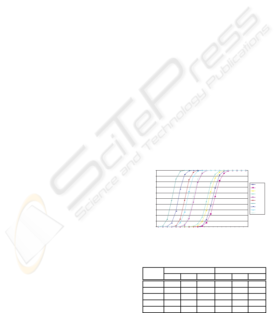
Figure 2, for instance, shows the Cumulative Den-
sity Function (CDF) of the NPV of all valid sequences
of the MMFs presented in Figure 1. The graphic pre-
sented in the picture was built from a sample of 5,000
observations generated by a Monte Carlo simulation
model. According to the information shown in the
graphic, under the criteria of probabilistic dominance,
the sequence ABDCE provides the best investment
alternative since its PDF dominates all the other se-
quences, i.e. for any given probability it will always
yield a better net present value.
0,00
0,10
0,20
0,30
0,40
0,50
0,60
0,70
0,80
0,90
1,00
500
525
550
575
600
625
650
675
700
725
750
775
800
825
850
875
900
925
950
975
1000
Thousands of US dollars
Comulative Probability
ABCDE
ABDCE
ABDEC
ADBCE
ADBEC
ADEBC
DEABC
DAEBC
DABEC
DABCE
Figure 2: CDF of valid sequences.
Table 3: Uncertain cash-flow elements of a set of MMFs.
MMF Investment Period Earnings
Min ML Max Min ML Max
A -48 -50 -55 40 45 50
B -30 -40 -50 50 60 70
C -15 -20 -25 30 35 40
D -48 -50 -54 40 50 60
E -40 -60 -70 25 30 35
ICEIS 2008 - International Conference on Enterprise Information Systems
26

Due to the exponential nature of the problem, the
method of sampling all valid sequences is unfeasi-
ble. For a set of n MMFs one may have do exam-
ine n! sequences. Therefore, an approximative heuris-
tic may have to be used. Denne and Cleland-Huang
(Denne and Cleland-Huang, 2003) suggest the use of
an heuristic algorithm which they have named “Incre-
mental Funding Method” (IFM). Also, because it is
not always the case that one comes across a dominat-
ing sequence when solving the problem of finding the
sequence of MMFs that yields the best return on in-
vestment, one needs a procedure for decision making
under uncertainty.
Both the heuristic algorithm and the generation of
data for the process of decision making under uncer-
tainty are addressed by the method described in the
next section.
4 THE METHOD
The method for obtaining an approximate solution to
the optimal order of execution of a software project
consists of the following steps:
1. Partition the product to be developed into a set of
n MMFs.
2. Define the precedence relations among the
MMFs.
3. Estimate the PDF of each cash-flow element asso-
ciated with each MMF.
4. Calculate the number of scenarios (NS) that must
be generated in order to obtain an estimate of the
probability of a given sequence being chosen by
the heuristic procedure, such that the error of its
the estimated CDF is kept below a certain value
under a required confidence level (Knuth, 1998).
5. Repeat the the procedure below NS times:
(a) obtain one scenario consisting of sampled val-
ues for each cash flow element of each MMF.
(b) apply an heuristic procedure for finding and
recording the sequence which maximizes the
NPV of the scenario.
6. Let SVS be the set of sequences generated in step
5. Obtain the PDF and CDF of the NPV of each
selected sequence by running a second set of NS
scenarios for each element of SVS. It is important
to notice that, in some cases, it may be necessary
to select a subset of SVS in order to reduce the
number of candidate sequences.
7. Apply a decision criteria for selecting the pre-
ferred sequence given a set the NPV of the se-
lected sequences. Two basic approaches can be
utilized: the direct choice and certainty equiva-
lent(Holloway, 1979). The direct choice utilizes
the CDF and the PDF of the NPV of each se-
quence in order to understand the uncertainty and
evaluate the risk. Outcome and probabilistic dom-
inance can used in this case.The certainty equiv-
alent approach establish an equivalence between
uncertain events and a certain value. This process
simplifies decision making by the removal of un-
certainty.
5 AN EXAMPLE
According to Benjamin Franklin (1706 - 1790), one
of the Founding Fathers of the United States: “A good
example is the best sermon”. As a result, this section
starts with an example of the algorithm presented in
Section 4.
5.1 Partition the Product
Consider a software S that can be divided into six
MMFs. Also, allow for the existence of three soft-
ware units that are essential for the implementation of
one or more of those MMFs, but that returns no rev-
enue.
5.2 Define the Precedence Relation
Figure 3, borrowed from (Denne and Cleland-Huang,
2003), shows the precedence graph of the MMFs and
AEs . In that figure A, B, ·· · , F are MMFs and 1, 2
and 3 are AEs.
1 A B
3
F
Start Finish
C
2 D
E
Figure 3: The precedence graph of the MMFs and AEs of
software S.
5.3 Define the PDF of Cash Flow
Elements
Table 4 presents the average present value of dis-
counted cash flow of the MMFs of software S, con-
sidering a discount rate of 2.4% per time period. In
this example, each cash-flow element bears an uncer-
tainty of 25%. Therefore, if MMF A is implemented
DEFINING THE IMPLEMENTATION ORDER OF SOFTWARE PROJECTS IN UNCERTAIN ENVIRONMENTS
27
in the first period it requires an initial investment be-
tween
−250 thousand (−200− 50)
and
-150 thousand (−200+ 50).
Table 4: The mean value of the cash flow elements.
Period MMF
A B C D E F
1 245 2,142 2,298 1,080 876 1,238
2 239 1,941 2,030 935 692 1,119
3 233 1,745 1,769 793 512 1,003
4 228 1,554 1,514 654 337 889
5 223 1,367 1,265 519 165 778
6 217 1,185 1,021 386 -2 670
7 206 1,007 784 257 -165 564
8 189 833 563 131 -325 461
9 167 664 368 20 -457 360
10 139 498 199 -77 -563 261
11 106 336 56 -159 -643 165
12 67 196 -63 -227 -698 71
13 24 77 -158 -282 -729 -21
14 -25 0 -229 -323 -735 -80
15 -78 -78 -277 -346 -484 -138
The same procedure can be applied to define the
discounted cash-flow of the AEs, using the same dis-
count rate of 2.4% per period.
5.4 Sample Cash Flow Streams
With the support of a Monte Carlo simulation tool
a sample of the discounted cash flow containing
5,000 observations is generated, using the look-ahead
heuristic proposed by Denne and Cleland-Huang
(Denne and Cleland-Huang, 2003).
It is important to note that because software S
yields a total of nine software units, potentially there
is a total of 362,880 = 9! MMF sequences whose NPV
has to be calculated. The heuristic reduces the num-
ber of sequences to four. The results are presented in
Table 5.
Table 5: Results of the Monte Carlo Simulation with a 25%
uncertainty.
Sequences Statistics
Freq. Min Max Mean Std.
Dev.
1ABC3F2DE 4,800 2,325 3,009 2,649 96
2DE3F1ABC 172 1,931 2,523 2,253 87
3F1ABC2DE 22 1,651 2,305 1,933 82
2DE1ABC3F 6 2,983 2,983 2,652 93
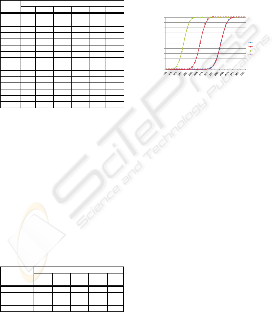
5.5 Obtain the CDF of the Selected
Sequences
Because the number of sequences is rather small (4
sequences), all are selected. A new 5,000 sample is
collected to reach the required error margin, within a
confidence interval, for the CDF of the NPV for the
implementation sequence. Figure 4 shows these re-
sults.
0,0
0,1
0,2
0,3
0,4
0,5
0,6
0,7
0,8
0,9
1,0
Comulative
Probability
Thousandsof US dollars
1ABC3F2DE
2DE3F1ABC
3F1ABC2EF
2DE1ABC3F
Figure 4: CDF of selected sequences.
5.6 Apply Decision Criteria
It should be noted that sequence 1ABC3F2DE,
which presents the best results under the mean
value (see (Denne and Cleland-Huang, 2003)),
and 2DE3F1ABC are outperformed by sequences
1AEC3F2DE and 2DE1ABC3F, which yield equiv-
alent value to business and are the optimal choices
under the uncertainties facing the project. A Wald-
Wolfowitz run test, with a 95% confidence interval,
does support these claims (Hill and Lewicki, 2005).
6 CONCLUSIONS
This article presents a method for maximizing the fi-
nancial return on investment in software projects. The
method considers that investment is maximized if the
software is divided into smaller software units, where
some of them have marketable value and others do
not. However, as the latter is essential for the devel-
opment of the former, the investment necessary to de-
velop such units influences the return on investment
yielded by the software and must be taken into ac-
count.
The method, which is based upon Monte Carlo
simulation, extends the ideais presented by (Denne
and Cleland-Huang, 2003; Denne and Cleland-
Huang, 2004; Cleland-Huang and Denne, 2005), al-
lowing for uncertain cash-flow streams, which are
ICEIS 2008 - International Conference on Enterprise Information Systems
28

so common in software projects and can actually be
found in many other kinds of projects.
The case study presented in the article shows that
results obtained taking uncertainty into account can
be very different from the ones assuming a known
cash-flow stream. Therefore, the investment made on
software must take uncertainty into account, specially
in the turbulent and globalized world where software
development takes place these days.
REFERENCES
Cleland-Huang, J. and Denne, M. (2005). Financially in-
formed requirements prioritization. In Proceedings of
the 27th international Conference on Software Engi-
neering, pages 710 – 711, St. Louis, MO, USA. As-
sociation for Computing Machinery (ACM) and ACM
Special Interest Group on Software Engineering (SIG-
SOFT), ACM.
Denne, M. and Cleland-Huang, J. (2003). Software by Num-
bers: Low-Risk High-Return Development. Prentice
Hall.
Denne, M. and Cleland-Huang, J. (2004). The incremental
funding method: Data driven software development.
IEEE Software, 21(3):39–47.
Germain, E. and Robillard, P. N. (2005). Engineering-based
processes and agile methodologies for software devel-
opment: a comparative case study. Journal of Systems
and Software, 75(1-2):17–27.
Hill, T. and Lewicki, P. (2005). Statistics: Methods and
Applications. StatSoft, Inc.
Holloway, C. A. (1979). Decision Making Under Uncer-
tainty: Models and Choices. Prentice Hall.
Hubbard, D. W. (2007). How to Measure Anything: Finding
the Value of “Intangibles” in Business. John Wiley &
Sons.
Knuth, D. E. (1998). The Art of Computer Programming:
Seminumerical Algorithms. Addison Wesley.
Kotler, P. and Armstrong, G. (2007). Principles of Market-
ing. Prentice Hall, 12
th
edition.
Kotz, S. and van Dorp, J. R. (2004). Beyond Beta: Other
Continuous Families Of Distributions With Bounded
Support And Applications. World Scientific Publish-
ing Company.
Little, T. (2004). Value creation and capture: A model of the
software development process. IEEE SOFTWARE.
Joint Task Force (2005). Computing curricula 2005: The
overview report. Technical report, The Associantion
for Computing Machinery (ACM), The Association
for Information Systems (AIS) and The Computer So-
ciety (IEEE-CS). Information available in the In-
ternet at www.acm.org/education/curricula.html. Site
last visited on October 28
th
, 2007.
Rashid, A., Moreira, A., and Ara´ujo, J. (2003). Modu-
larisation and composition of aspectual requirements.
In Proceedings of the 2
nd
International Conference
on Aspect-oriented Software Development, pages 11
– 20, Boston, Massachusetts, USA. Northeastern Uni-
versity, ACM.
Robert, C. P. and Casella, G. (2005). Monte Carlo Statisti-
cal Methods. Spinger-Verlag, 2
nd
edition.
Scott, D. (2006). I.T. Wars: Managing the Business-
Technology Weave in the New Millennium. BookSurge
Publishing.
Thomas, J. S. and Duffy, D. E. (2004). The Statistical Anal-
ysis of Discrete Data. Springer-Verlag, 1
st
edition.
Verhoef, C. (2005). Quantifying the value of IT-
investments. Science of Computer Programming,
56:315–342.
Vose, D. (2000). Risk Analysis: A Quantitative Guide. John
Wiley & Sons, 2
nd
edition.
DEFINING THE IMPLEMENTATION ORDER OF SOFTWARE PROJECTS IN UNCERTAIN ENVIRONMENTS
29
