
A NEW LEARNING ALGORITHM FOR CLASSIFICATION IN
THE REDUCED SPACE
Luminita State
Department of Computer Science, University of Pitesti, Pitesti, Romania
Catalina Cocianu, Ion Rosca
Department of Computer Science, Academy of Economic Studies, Bucharest, Romania
Panayiotis Vlamos
Department of Computer Science, Ionian University, Corfu, Greece
Keywords: Feature extraction, informational skeleton, principal component analysis, unsupervised learning, cluster
analysis.
Abstract: The aim of the research reported in the paper was twofold: to propose a new approach in cluster analysis
and to investigate its performance, when it is combined with dimensionality reduction schemes. Our attempt
is based on group skeletons defined by a set of orthogonal and unitary eigen vectors (principal directions) of
the sample covariance matrix. Our developments impose a set of quite natural working assumptions on the
true but unknown nature of the class system. The search process for the optimal clusters approximating the
unknown classes towards getting homogenous groups, where the homogeneity is defined in terms of the
“typicality” of components with respect to the current skeleton. Our method is described in the third section
of the paper. The compression scheme was set in terms of the principal directions corresponding to the
available cloud. The final section presents the results of the tests aiming the comparison between the
performances of our method and the standard k-means clustering technique when they are applied to the
initial space as well as to compressed data.
1 INTRODUCTION
Basically, a cluster analysis method can be viewed
as an unsupervised learning technique and usually it
is a pre-processing step in solving a pattern
recognition problem. The objective of cluster
analysis is simply to find a convenient and valid
organization of the data, not to establish rules for
separating future data into categories.
The most intuitive and frequently used criterion
function in partitional clustering techniques is the
squared error criterion, which tends to work well
with isolated and compact clusters. The k-means is
the simplest and most commonly used algorithm
employing a squared error criterion (McQueen
1967).
The aim of the present paper is to propose a new
kind of approach in cluster analysis. Our attempt is
based on group skeletons defined by a set of
orthogonal and unitary eigen vectors (principal
directions) of the sample covariance matrix.
According to the well known result established by
Karhunen and Loeve, a set of principal directions
corresponds to the maximum variability of the
“cloud” from metric point of view, as well as from
informational point of view. The performance of
our algorithm is tested against the k-means method
in the initial representation space as well as in the
reduced space of features given by principal
directions. In our approach the skeleton of a group is
represented by the principal directions of this
sample.
Since similarity is fundamental to the definition
of a cluster, a measure of the similarity between two
155
State L., Cocianu C., Rosca I. and Vlamos P. (2008).
A NEW LEARNING ALGORITHM FOR CLASSIFICATION IN THE REDUCED SPACE.
In Proceedings of the Tenth International Conference on Enterprise Information Systems - AIDSS, pages 155-160
DOI: 10.5220/0001676501550160
Copyright
c
SciTePress

patterns drawn from the same feature space is
essential to most clustering procedures. It is most
common to calculate the dissimilarity between two
patterns using a distance measure defined on the
feature space. The dissimilarity measure used in our
method is defined in terms of the Euclidian distance
between the group skeletons.
Our developments impose a set of quite natural
working assumptions on the true but unknown
nature of the class system. The search process for
the optimal clusters approximating the unknown
classes towards getting homogenous groups, where
the homogeneity is defined in terms of the
“typicality” of components with respect to the
current skeleton. Our method is described in the
third section of the paper. The final section presents
the results of the tests aiming to derive comparative
conclusions abut the performances of our method
and the k-means in the initial representation space
and the reduced spaces.
2 A SKELETON-BASED
DISSIMILARITY MEASURE
Let us assume that the recognition task is formulated
as a discrimination problem among M classes or
hypothesis. We denote by H the set of hypothesis.
The Bayesian point of view is usually expressed in
terms of an a priori probability distribution
ξ
on H,
where for each
Hh ∈
,
()
h
ξ
stands for the
probability of getting an example coming from class
h.
In the supervised framework, for each class
h , a
sample of examples coming from this class
() () ()
{}
h
h
N
hh
XXX ,...,,
21
is available. We denote by
(
)
(
)
(
)
{
}
U
Hh
h
h
N
hh
XXX
∈
=ℵ ,...,,
21
,
∑
∈
=
Hh
h
NN .
Therefore, each element of
ℵ can be viewed as
a tagged component, where the tag is the label of the
provenience class. For each class, the sample mean
() ()
∑
=
=
h
N
i
h
i
h
h
h
N
X
N
1
1
μ
can be viewed as a template or
prototype for the class which typicality depends on
the variability existing within the sample. The
components of the sample covariance matrix
() () ()
()
() ()
()
∑
=
−−
−
=∑
h
N
i
T
h
h
N
h
i
h
h
N
h
i
h
h
h
N
XX
N
1
1
1
μμ
express the global correlations between the attributes
measured in the representation space with respect to
the sample coming from class
h. Therefore, the
variability degree of each class
h is usually
expressed in terms of a real valued function f of
(
)
h
h
N
μ
and
(
)
h
h
N
∑ .
The global prototype and overall sample
covariance matrix are given by the mixture of
(
)
(
)
(
)
{
}
Hh
h
h
N
h
h
N
∈∑ ,,
μ
with respect to
ξ
, that is
()
(
)
∑
∈
=
Hh
h
h
N
N
h
μξμ
(1)
()
(
)
∑
∈
∑=∑
Hh
h
h
N
N
h
ξ
(2)
The value of
(
)
(
)
(
)
h
h
N
h
h
N
f ∑,
μ
represents a measure
of the overall variability existing in the “cloud”
ℵ
.
In cases the probability distribution
ξ
is unknown, it
is usually estimated by the relative frequencies, that
is, for each
Hh
∈
,
()
N
N
h
h
≈
ξ
.
In the unsupervised case, the available data is
represented by
{
}
N
XXX ,...,,
21
=
ℵ
, an untagged set
of examples of a certain volume
N, coming from the
classes of
H. The task is to develop suitable
algorithm to identify the groups of examples coming
from each class. Usually, these groups are referred
to as clusters. The problem is usually solved using a
conventional dissimilarity measure defined in terms
of the measured attributes, whose value for each pair
of examples expresses in which extent these
examples “are different”.
In our attempt we define a dissimilarity measure
to express the fitness degree of an element with
respect to a cluster by a function expressing a
measure of disturbance of cluster structure induced
by the decision of including this element into the
given cluster. Our developments are based on the
following set of working assumption
.
1. Each data of
ℵ
is the realization of a certain random
vector corresponding to an unique but unknown
class of the set
H. Let HM = , wher H stands for
the number of elements of
H. We assume that M is
known.
2. The classes are well separated in the
representation space
R
n
.
3. For each class
Hk
∈
, it is available an
example
k
P coming from this class
The idea behind our approach is to use the
skeletons as basis in developing the search for
M-
homogenous groups starting with
M
PPP ,..,,
21
as
initial
seeds. The closeness degree of a particular
data
X to a cluster C is measured by the distance
between skeletons of
C and
{}
XC ∪ . From
ICEIS 2008 - International Conference on Enterprise Information Systems
156

intuitive point of view, in case C includes mostly
elements coming from the same class
k, C results
homogenous, and for
X coming from k, the distance
between
C and
{}
XC ∪ is negligible.
The search process allots/re-allots data to the
current set of clusters aiming to produce
M clusters
as homogenous as possible. The computation of the
distance between the skeletons of
C and
{
}
XC ∪
can be simplified using first order approximation as
follows. If
{}
r
XXXC ,...,,
21
= , the sample means
and the sample covariance matrices of
C and
{}
XC ∪ are given by,
∑
=
=
r
i
ir
X
r
1
1
μ
(3)
X
r
r
r
rr
1
1
1
1
+
+
+
=
+
μμ
(4)
()()
∑
=
−−
−
=Σ
r
i
T
ririr
XX
r
1
1
1
μμ
(5)
()()
r
T
rrrr
r
XX
r
Σ−−−
+
+Σ=Σ
+
1
1
1
1
μμ
(6)
Let
r
n
rr
λλλ
≥≥≥ ...
21
be the eigen values and let
r
n
r
ψψ
,...,
1
be the orthonormal eigen vectors of
r
Σ
.
In case the eigen values of
r
Σ are pairwise distinct,
the following first order approximations of the eigen
values and eigen vectors of
1+
Σ
r
hold,
() ()
r
ir
T
r
i
r
ir
T
r
i
r
i
r
i
ψΣψψΣψ
1
1
+
+
=Δ+=
λλ
(7)
()
∑
≠
=
+
−
Δ
+=
n
ij
j
r
j
r
j
r
i
r
ir
T
r
j
r
i
r
i
1
1
ψ
ψΣψ
ψψ
λλ
(8)
where
rrr
Σ−Σ=ΔΣ
+1
.
The closeness degree of
X to C is defined by
()
()
∑
=
+
−=Ψ=
n
j
r
j
r
j
r
n
XDCXD
1
2
1
1
,,
ψψ
,(9)
where
2
stands for the Euclidian norm in R
n
.
Obviously, the performance in time of any
unsupervised classification method is strongly
dependent on the dimension of the input data.
Consequently, the decrease of the input data
dimension by some sort of compression scheme
could become worth from time efficiency point of
view. However, any dimensionality reduction
scheme implies missing information therefore the
accuracy could become dramatically affected.
Therefore, in real cluster analysis task, getting a
tradeoff between accuracy and efficiency by
selecting the most informational features becomes
extremely important. In case of unsupervised cluster
analysis, the features have to be extracted
exclusively from the available data.
3 THE DESCRIPTION OF THE
PROPOSED CLUSTER
ANALYSIS SCHEME
The aim of this section is to present a new
unsupervised classification scheme (SCS) based on
cluster skeletons. The input is represented by:
¾ the data
{
}
N
XXX ,...,,
21
=
ℵ
to be classified;
¾ M, the number of clusters;
¾ the set of initial seeds,
M
PP ,...,
1
.
Parameters:
¾ n, the dimension of input data;
¾
θ
, the threshold value to control the cluster
size;
(
)
1,0
∈
θ
;
¾ nr, the threshold value to control the cluster
homogeneity;
¾ Cond, the stopping condition, expressed in
terms of the threshold value
NoRe, for the
number of re-allotted data;
¾
ρ
, the control parameter,
()
1,0∈
ρ
, to control
the fraction of “disturbing” elements identified
as outliers and removed from clusters.
P1. The Generation of the Initial Clusters,
{
}
00
2
0
1
0
,...,,
M
CCC=C ,
{}
kk
PC =
0
, Mk ,...,1=
The initial clusters are determined around the seeds
using a minimum distance criterion.
P2. Compute the System of Cluster Skeletons,
{
}
t
M
tt
SS ,...,
1
=S ,where
{}
t
nk
t
k
t
k
t
k
S
,2,1,
,...,,
ψψψ
= is
the skeleton of the cluster
k at the moment t. We
denote by
{
}
it
nk
it
k
it
k
it
k
S
,
,
,
2,
,
1,
,
,...,,
ψψψ
= the skeleton of
{
}
i
t
k
XC ∪
, Ni
≤
≤
1 .
P3.
REPEAT
t=t+1;
1−
=
tt
SS
;
1−
=
tt
CC ;
{Compute the new cluster system
{
}
t
M
ttt
CCC ,...,,
21
=C
}
for Mk ,...,1
=
{compute the cluster
t
k
C }
=
t
k
C Ø;
P3.1.
for Ni ,1=
A NEW LEARNING ALGORITHM FOR CLASSIFICATION IN THE REDUCED SPACE
157
for Mcl ,1= compute
()
t
cli
SXD ,
;
endfor
compute
()
t
cli
Mcl
SXDl ,minarg
1 ≤≤
= ;
if k=l then
{
}
i
t
k
t
k
XCC ∪← ;
{
}
i
t
p
t
p
XCC \← ,
where
p is such that
t
pi
CX ∈
endif
endfor
P3.2. {test the homogeneity of
t
k
C
}
compute
t
k
c the center of
t
k
C ;
∑
∈
=
t
k
CX
t
k
t
k
X
C
c
1
re-compute
t
k
S
, the skeleton of
t
k
C
;
compute
⎪
⎭
⎪
⎬
⎫
⎪
⎩
⎪
⎨
⎧
−>−∈=
∈
22
1
max
t
k
t
k
CX
t
k
t
k
cXcXCXF
θ
;
compute
(
)
(
)
{
}
t
j
t
k
t
k
SXDSXDkjCXF ,,,
2
>≠∃∈= ;
if
nrFF >∪
21
then
t
k
C is not homogenous
else
t
k
C is homogenous
endif
P3.3.
{extend
t
k
C in case it is homogenous by
adding the closest elements }
if
t
k
C is homogenous then
for each
t
k
CX \ℵ∈
for Mcl ,...,1= compute
()
t
cl
SXD ,
endfor
compute
()
t
cl
Mcl
SXDl ,minarg
1 ≤≤
= ;
if k=l then
{}
i
t
k
t
k
XCC ∪←
,
{
}
i
t
p
t
p
XCC \← ,
where p is such that
1−
∈
t
pi
CX
endif
endfor
else
{
t
k
C is not homogenous }
Felim
ρ
= ;
compute SET1 the set of the most ”disturbing” elim
elements from F (identified as outliers with respect
to
t
k
C )
{elements of maximum distance to
t
k
S }
for each
1SETX ∈
for Mcl ,...,1= compute
()
t
cl
SXD , ;
endfor
compute
()
t
cl
Mcl
SXDl ,minarg
1 ≤≤
= ;
if l<>k then
{
}
XCC
t
l
t
l
∪← ;
{}
XCC
t
k
t
k
\← ;
endif
endfor
endif
P3.4.
re-compute
t
k
S
, the skeleton of the new
t
k
C
;
P3.5.
{re-allot the elements of
t
k
t
k
CC \
1−
}
for each
t
k
t
k
CCX \
1−
∈
for
Mcl ,...,1
=
compute
()
t
cl
SXD ,
endfor
compute
()
t
cl
Mcl
SXDl ,minarg
1 ≤≤
= ;
{
}
XCC
t
l
t
l
∪←
;
endfor
P3.6.
Compute the new set of skeletons
t
S
{the computation of
t
k
C is over}
endfor
UNTIL
Cond
The use of the previously presented
classification scheme combined with a compression
applied to reduce data dimensionality can be
developed either by compressing with respect to the
overall principal directions (variant 1) or with
respect to the principal directions of each initial
cluster (variant 2).
Set the value of m,
nm <
<
1 ,
Variant 1. The overall compression
1.1. Determine the principal directions of the
initial data
ℵ
using
N
μ
and
N
∑ given by (1) and (2).
1.2. Get the m-dimensional representation
m
ℵ
of
ℵ
by projecting the components of ℵ on the m-
dimensional subspace represented by the first m
principal directions
1.3. Apply the classification scheme to
m
ℵ .
Variant 2. Cluster compression
2.1. Apply P1 to get the initial system of
clusters
{
}
00
2
0
1
0
,...,,
M
CCC=C
2.2. Determine the principal directions for each
cluster of
0
C .
2.3. Get the compressed m-dimensional versions
of data by compressing each element with respect to
systems of principal directions corresponding to the
cluster it belongs to.
ICEIS 2008 - International Conference on Enterprise Information Systems
158

2.4. Get
m
ℵ as the union of the resulted m-
dimensional versions.
2.5. Apply the classification scheme to
m
ℵ
4 EXPERIMENTAL
PERFORMANCE
EVALUATION OF THE
PROPOSED ALGORITHM
A series of tests were performed in order to derive
conclusions about the performance of our method as
well as to test its performance against the k-means
algorithm. The stopping condition Cond=True holds
if IN the current iteration resulted at most NoRe re-
allots; in our tests NoRe was set to NoRe=10. The
tests were performed for M=4, the data being
randomly generated by sampling from normal
repartitions. Some of the repartitions were selected
to correspond to “well separated” classes some
others being generated to correspond to “bad
separated” subsets of classes, the working
assumption 2 not being necessarily fulfilled.
In order to obtain conclusions concerning
algorithm sensitivity to data dimensionality, several
tests were performed for n=2, n=4, n=6, n=8, n=10.
The tests on our algorithm and k-means pointed out
the following conclusions.
1. In cases when there is a natural grouping
tendency in data, the initial system of skeletons is pretty
close to the true one. In these cases, our algorithm gets
stabilized in a small number of iterations.
2. In case of data of relatively small size, the
number of misclassified components by our
algorithm is significantly less than the number of
misclassified data using k-means.
3. In cases of data of relatively small size, the
performance of k-means algorithm in identifying the
cluster structures is significantly less than the
performance of our method.
4. The k-means algorithm is significantly more
sensitive to data dimensionality, its performance
decreasing dramatically as the dimension n
increases.
5. In case of large sample sizes, the performance
of our method is comparable to the performance of
k-means.
Several tests were performed for “well
separated” classes, relatively “separated” and “bad
separated” respectively. In all tests, the performance
of k-means proved moderated, while our method
managed to identify the class structures and to
correctly classify most of data. The closeness degree
between the classes is computed in terms of the
Mahalanobis distance.
Some of the results are reported below.
A. M=4, n=4 and relative small size data. The
classes are weakly separated , the values of the
Mahalanobis distances are
⎟
⎟
⎟
⎟
⎟
⎠
⎞
⎜
⎜
⎜
⎜
⎜
⎝
⎛
09349.3691386.8466289.351
9349.36903931.2655993.214
1386.8463931.26501542428
6289.3515993.21415424280
.
.
In this case, the classification scheme managed
to discover the true structure of data in the initial
space, but using the compression for
3
=
m and
2
=
m its performance degraded dramatically. The k-
means algorithm did not manage to identify the
existing structure in the initial space. Some of he
results are summarized in the following table.
Note that for the samples
S
1
, S
2
and S
4
the k-
means failed to identify the cluster structures.
Table 1: The comparison of our method against k-means.
The sample
S
1
S
2
S
3
S
4
Number of
misclassified examples
by our method
0 2 0 0
Number of
misclassified examples
by k-means
276 253 19 311
N
umber of iterations 3 2 2 2
B. M=4, n=4 and relative small size data. In this
case, the true classes are better separated. The values
of the Mahalanobis distances are
⎟
⎟
⎟
⎟
⎟
⎠
⎞
⎜
⎜
⎜
⎜
⎜
⎝
⎛
06171.019.19733.0
6171.002827.04139.0
19.12827.004183.0
9733.04139.04183.00
10
3
In this case good results were obtained by
applying the proposed classification scheme in the
initial space as well as for m=3. All tests proved
better performances of our method as compared to k-
means. Some of the results are summarized in the
following table.
A NEW LEARNING ALGORITHM FOR CLASSIFICATION IN THE REDUCED SPACE
159
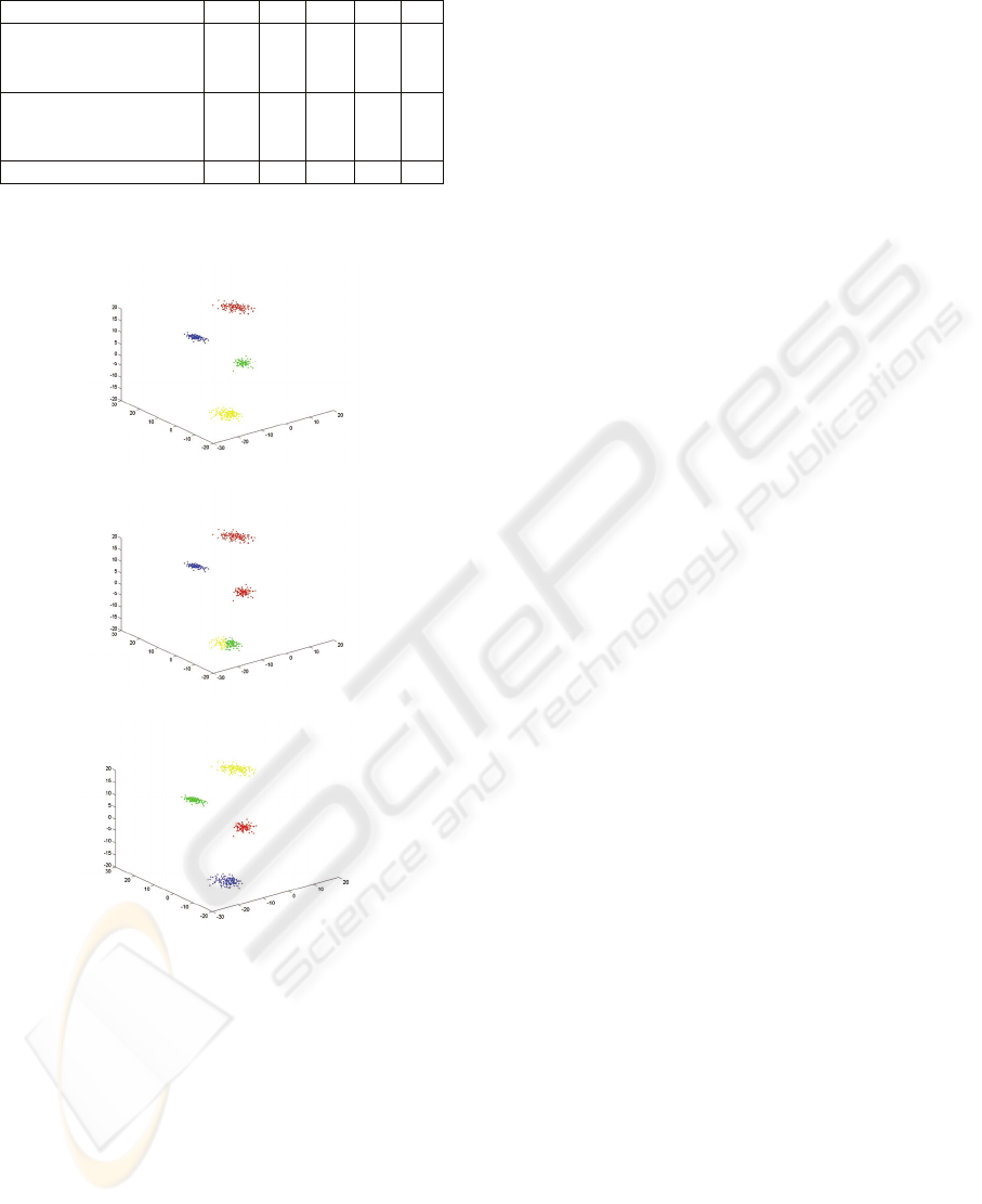
Table 2: The comparison of our method against k-means.
The sample
S
1
S
2
S
3
S
4
S
5
Number of
misclassified examples
by our method
0 0 0 0 0
Number of
misclassified examples
by k-means
315 0 325 31
8
0
N
umber of iterations 2 2 3 2 2
The 3-dimensional representations of data
corresponding to S are depicted in figure 1.
a. The true system of classes
b. The clusters produced by k-means algorithm
c. The clusters computed by our method
Figure 1: The results on the sample S
1.
REFERENCES
Cocianu, C., State, L., Rosca, I., Vlamos, P, 2007. A New
Adaptive Classification Scheme Based on Skeleton
Information. In
Proceedings of ICETE-SIGMAP
2007
, Spain.
Diamantaras, K.I., Kung, S.Y., 1996.
Principal
Component Neural Networks: theory and applications
,
John Wiley &Sons
Everitt, B. S., 1978.
Graphical Techniques for
Multivariate Data
, North Holland, NY
Fayyad, U.M., Piatetsky-Shapiro, G., Smyth, P., and
Uthurusamy, R., 1996.
Advances in Knowledge
Discovery and Data Mining
, AAAI Press/MIT Press,
Menlo Park, CA.
Goldberger, J., Roweis, S., Hinton, G., Salakhutdinov, R.,
2004. Neighborhood Component Analysis. In
Proceedings of the Conference on Advances in Neural
Information Processing Systems
Gordon, A.D. 1999.
Classification, Chapman&Hall/CRC,
2
nd
Edition
Hastie, T., Tibshirani, R., Friedman, J. 2001.
The Elements
of Statistical Learning Data Mining, Inference, and
Prediction.
Springer-Verlag
Hyvarinen, A., Karhunen, J., Oja, E., 2001.
Independent
Component Analysis
, John Wiley &Sons
Jain,A.K., Dubes,R., 1988.
Algorithms for Clustering
Data
, Prentice Hall,Englewood Cliffs, NJ.
Jain, A.K., Murty, M.N., Flynn, P.J. 1999. Data clustering:
a review.
ACM Computing Surveys, Vol. 31, No. 3,
September 1999
Liu, J., and Chen, S. 2006. Discriminant common vectors
versus neighborhood components analysis and
Laplacianfaces: A comparative study in small sample
size problem.
Image and Vision Computing 24 (2006)
249-262
MCQueen, J. 1967. Some methods for classification and
analysis of multivariate observations. In
Proceedings
of the Fifth Berkeley Symposium on Mathematical
Statistics andProbability
, 281–297.
Panayirci,E., Dubes,R.C., 1983. A test for
multidimensional clustering tendency.
Pattern
Recognition
,16, 433-444
Smith,S.P., Jain,A.K., 1984. Testing for uniformity in
multidimensional data, In
IEEE Trans.`Patt. Anal.`
and Machine Intell.
, 6(1),73-81
State L., Cocianu C. 1997. The computation of the most
informational linear features,
Informatica Economica,
Vol. 1, Nr. 4
Ripley, B.D. 1996. Pattern Recognition and Neural
Networks
, Cambridge University Press, Cambridge.
ICEIS 2008 - International Conference on Enterprise Information Systems
160
