MAXIMIZING THE BUSINESS VALUE OF SOFTWARE PROJECTS

A Branch & Bound Approach

Antonio Juarez Alencar, Eber Assis Schmitz,

Enio Pires de Abreu, Marcelo Carvalho Fernandes

Graduate Program in Informatics, Institute of Mathematics and Electronic Computer Center

Federal University of Rio de Janeiro, Rio de Janeiro, Brazil

Armando Leite Ferreira

The COPPEAD School of Business, Federal University of Rio de Janeiro, Rio de Janeiro, Brazil

Keywords:

Branch & Bound, Minimum Marketable Feature, Incremental Funding Method, Project Management and

Business Performance.

Abstract:

This work presents a branch & bound method that allows software managers to determine the optimum order

for the development of a network of dependent software parts that have value to customers. In many different

circumstances the method allows for the development of complex and otherwise expensive software from a

relatively small investment, favoring the use of software development as a means of obtaining competitive

advantage.

1 INTRODUCTION

In today’s highly-competitive globalized market,

software development projects are unlikely to be

funded unless they yield clearly-deﬁned low-risk

value to business (McManus, 2003). Moreover,

in such competitive markets stakeholders frequently

call for shorter investment payback time, product-

development faster time-to-market, and a business ar-

chitecture with improved operational agility (Lam,

2004; Helo et al., 2004; Whittle and Myrick, 2005).

All of this requires new approaches to software

project development (Jorgenson et al., 2003; High-

smith, 2002).

To deal with this situation both academics and

software developers have strongly emphasized the

need for methods, concepts and tools that favor the

early delivery of functional parts of software sys-

tems that are valued by customers (Abacus et al.,

2005; Nord and Tomayko, 2006). In this sense, the

Incremental Funding Method, or IFM, is a ﬁnan-

cially responsible approach to requirement prioriti-

zation that increases the value creation of software

projects (Denne and Cleland-Huang, 2004a; Denne

and Cleland-Huang, 2004b).

The IFM groups requirements into self-contained

interdependent software units that create value to

business in one or several of the following areas:

• Competitive Differentiation - the software unit al-

lows the creation of service or product features

that are valued by customers and that are different

from anything else being offered in the market;

• Revenue Generation - although the software unit

does not provide any unique valuable features to

customers, it does provide extra revenue by offer-

ing the same quality as other products in the mar-

ket for a better price;

• Cost Savings - the software unit allows business

to save money by making one or more business

processes cheaper to run;

• Brand Projection - by building the software unit

the business projects itself as being technologi-

cally advanced; and

• Enhanced Customer Loyalty - the software unit

inﬂuences customers to buy more, more fre-

quently or both.

Moreover, the total value brought to an organiza-

tion by a software consisting of several interdepen-

dent units, each one with its own cash ﬂow and prece-

dence restrictions, is highly dependent on the imple-

mentation order of these units.

162

Juarez Alencar A., Assis Schmitz E., Pires de Abreu Ê., Carvalho Fernandes M. and Leite Ferreira A. (2008).

MAXIMIZING THE BUSINESS VALUE OF SOFTWARE PROJECTS - A Branch & Bound Approach.

In Proceedings of the Tenth International Conference on Enterprise Information Systems - ISAS, pages 162-169

DOI: 10.5220/0001685801620169

 SciTePress

Therefore, the method includes a set of

polynomial-time sequencing strategies that helps

ﬁnding a suitable development schedule that im-

proves the overall value of projects, reduce initial

investments, or enhance other project metrics such as

time needed for a project to break even and payback

time (Denne and Cleland-Huang, 2004b; Denne and

Cleland-Huang, 2005).

However, the strategies proposed by the IFM does

not lead, in all circumstances, to the best possible

schedule, which can only be achieved, in the general

case, in an exponential time. Furthermore, in order

to allow the sequencing algorithm to run in a polyno-

mial time, the IFM requires that the development of

a software unit may depend upon the development of

no more than a single software unit.

This work presents a branch & bound method that

ﬁnds the schedule that maximizes the business value

of a software project and that imposes no restrictions

on the dependencies that may exist among software

units, making the method more attractive to be used

in the real world. Although, the branch & bound is an

exponential method, there are many circumstances in

which it can ﬁnd the best possible solution to an opti-

mization problem in a polynomial time. See (Liberti,

2003; Hillier and Lieberman, 2001) for an introduc-

tion to the branch & bound method.

The remaining of this paper is organized as fol-

lows. Section 2 presents a review of the principal con-

cepts and methods used in the article. Section 3 intro-

duced the branch & bound method with the help of an

example. The method is formalized in Section 4. Sec-

tion 5 discusses the implications of the method for dif-

ferent dimensions project management. Finally, Sec-

tion 6 presents the conclusions of this paper.

2 CONCEPTUAL FRAMEWORK

The self-contained units in which the IFM partitions a

software project are called Minimum Marketable Fea-

tures, or MMF for short, indicating that they contain

strongly-related software features that can be quickly

delivered and that are valued by customers (Steindl,

2005; Denne and Cleland-Huang, 2004b).

Although an MMF is a self-contained unit, it is

often the case that an MMF can only be developed

after other project parts have been completed. These

project parts may be either other MMFs or the archi-

tectural infrastructure, i.e. the set of basic features

that offers no direct value to customers, but that are

required by the MMFs.

The architecture itself can usually be decomposed

into self-contained deliverable elements. These el-

ements, called Architectural Elements or AEs for

short, enables the architecture to be delivered accord-

ing to demand, further reducing the initial investment

needed to run a software project. See (Rashid et al.,

2003) for directions on how software module and

architectural elements may be derived from require-

ments.

2.1 Cash Flow

After the MMFs and AEs have been identiﬁed, devel-

opers and business personnel collaborate to analyze

for each MMFs and AEs their estimated cost and ex-

pected revenues over a window of opportunity. See

(Hubbard, 2007) for a discussion on how these esti-

mates may be obtained in real-world projects. These

costs and revenues form a cash ﬂow that can be used

to estimate the total value of the software.

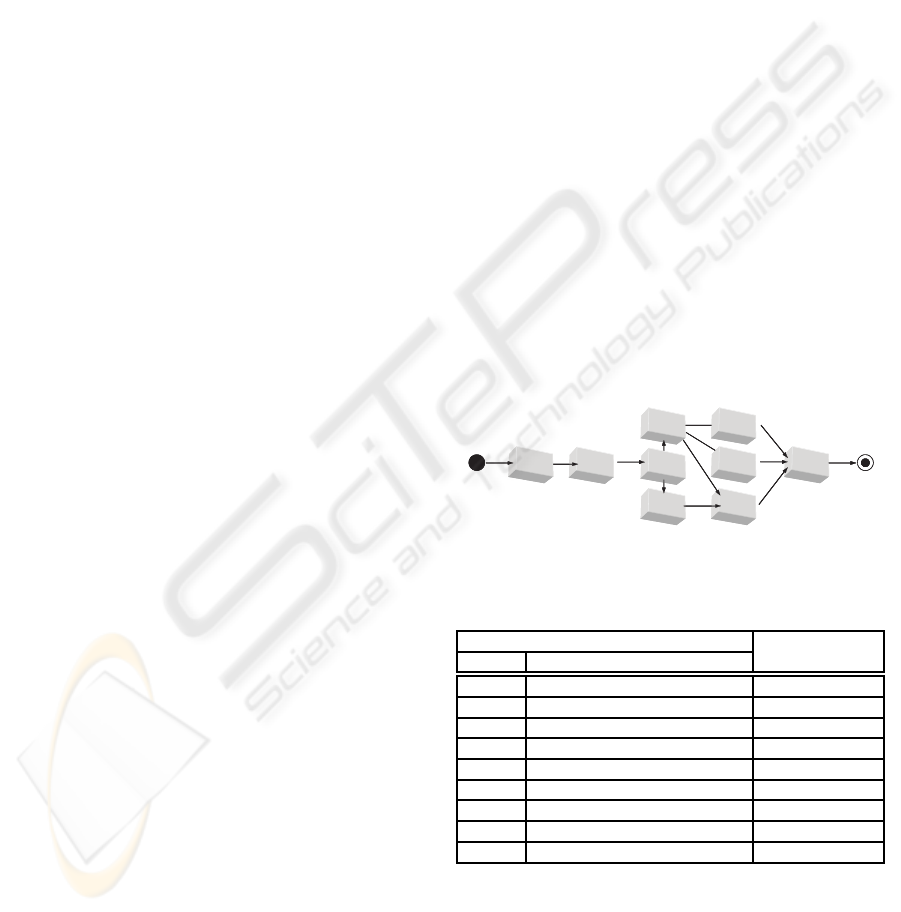
For example, Figure 1 presents a set of interdepen-

dents MMFs and AE’s. In that ﬁgure GIL is the ﬁrst

tool to be developed and CLM the last. Moreover, an

arrow connecting two activities such as PdS → Pc in-

dicates that the latter development efforts may only

start when the former has been completed and all the

necessary resources are available. Table 1 shows the

activity supported by each unit and whether they are

an MMF or an AE.

Start End

PsS

PdS

CLM

GIL

Start End

PsS

PdS

CLM

GIL

Figure 1: A precedence graph of project units.

Table 1: List of software units to be developed.

Tool Type of

Name Supported Activity Software Unit

GIL Graphical Interface Library AE

PdS Product Selection MMF

PsS Prospect Selection MMF

Pc Pricing MMF

CD Catalog Design MMF

LP Label Printing MMF

SC Stock Control MMF

CP Catalog Printing MMF

CLM Catalog Labeling & Mailing MMF

Table 2 shows the expected cash ﬂow for the set

of project units presented in Figure 1. In that table

periods are time interval of equal length, where an

investment is made or a revenue is earned.

In formal terms a window of opportunity P is a

set {p

, p

, ··· , p

} of time periods of equal length.

MAXIMIZING THE BUSINESS VALUE OF SOFTWARE PROJECTS - A Branch & Bound Approach

163

In Table 2, P = {1, 2, ··· , 12}. Also, the cash-ﬂow of

a project unit v

is given by cf(v

) and the cash ﬂow

element of v

in period p ∈ P is given by cf(v

, p). In

Table 2, cf(CD) at period 1, i.e. cf (CD, 1), is -70 and

cf(CD) in period 2, i.e. cf(CD, 2), is 20.

2.2 The Precedence Relationship

The development constraints between MMFs and

AEs can be represented by a directed acyclic graph

showing their precedence relationship. Figure 1 in-

troduces one of these graphs. In that graph, Start and

Finish are dummy units that take no time to be exe-

cuted and yield no cash ﬂows, signaling respectively

the beginning and end of a project.

In formal terms a precedence graph of project

units is a mathematical structure G(V, E) where:

• V = {v

, v

, · · · , v

} is a set of MMFs and AEs,

and

• E is a set of ordered pairs, such that if (v

, v

) ∈ E,

then v

depends on the completion of v

In the graph presented in Figure 1, V

= {Start, GIL,

PdS, ··· , CLM, End} e E

= {(Start, GIL), (GIL,

PdS), (PdS, Pc), ··· , (CP, CLM), (CLM, End)}. A

thorough introduction to graph theory can be found in

(Gross and Yellen, 2005).

2.3 Discounted Cash Flow

Because it is improper to perform mathematical op-

erations on monetary values without taking into ac-

count an interest rate, in order to compare the value of

different MMFs one has to resort to their discounted

cashﬂow (Fabozzi et al., 2006). In formal terms, the

net present value of a software unit v

whose develop-

ment starts at period t ∈ P is given by the sum o its

discounted cash ﬂows, i.e.

Table 2: The cash ﬂow of the project units in thousands of

US dollars.

Project Periods

Unit 1 2 3 ·· · 12

GIL -50 0 0 ·· · 0

PdS -40 20 20 ·· · 20

PsS -50 30 30 · ·· 30

Pc -30 15 15 ·· · 15

CD -70 20 20 ·· · 20

LP -20 5 5 ··· 5

SC -200 40 40 ··· 40

CP -50 15 15 ·· · 15

CLM -50 200 200 ·· · 200

npv(v, t) =

∑

j=t

cf(v, j −t +1)

(1+

100

)

where r is the discount rate and n is the last period

of the window of opportunity P. For example, if the

development of MMF CD starts in period 1, then its

NPV is

npv(CD, 1) =

−70

(1+

100

)

+ ·· · +

(1+

100

)

= $123

Table 3 shows the discounted cash-ﬂows of each

MMF in Figure 1, considering a 2% discount rate, at

different starting points within a window of opportu-

nity P. Note that the table considers only the ﬁrst nine

periods of the window of opportunity, as these are the

periods in which the software units are going to be

developed.

Table 3: The NPVs of the project units in thousands of US

dollars with a discount rate of 2%.

Project Periods

Unit 1 2 3 4 ·· · 9

GIL -49 -48 -47 -46 ·· · -42

PdS 153 134 116 98 ··· 15

PsS 239 211 184 157 ··· 31

Pc 115 101 87 74 ··· 11

CD 123 105 88 71 · ·· -10

LP 28 24 20 15 ··· -5

SC 188 153 119 86 ·· · -71

CP 95 81 68 55 ··· -6

CLM 1870 1679 1491 1307 ·· · 441

The reader should not be surprised that the dis-

counted cash-ﬂow of AE

in period 1 is -$49 thousand

and not -$50 as one could have naively expected. One

should keep in mind that although development ser-

vices are earned at the beginning of a period, they

are paid for upon delivered at the end of that pe-

riod, when, according to the discount rate, money is

worth slightly less than at the beginning of the period

(Fabozzi et al., 2006).

2.4 Net Present Value

Obviously, the value of a project depends upon the or-

der in which the software units are developed. For ex-

ample, if the development order of the software units

in Figure 1 is GIL → PdS → Pc → CD → PsS →

SC → CP → LP → CLM, than they yield a revenue

vpl(GIL, 1) + vpl(PdS, 2) + ··· +vpl(CLM, 9) =

−$49− $134+ ·· · + $441 = $853

ICEIS 2008 - International Conference on Enterprise Information Systems

164

However, if the development order is GIL → PdS →

Pc → CD → PsS → LP → SC → CP → CLM, than

they yield a revenue of $818.

Because not all sequences of software units neces-

sarily comply with the established precedence restric-

tions (see Figure 1), it is important to formally deﬁne

what a valid sequence of units is. In this sense a valid

sequence VS is an ordered set of software units such

that:

• All software units belong to the sequence and are

listed exactly once,

• Only one software unit can be in the implementa-

tion process at any given time period,

• The process of developing a software unit can

only start after its precedent units are completed,

• The ﬁrst software unit must start in the ﬁrst period

and

• Apart from the last, there is no time delay between

the end of the implementation of a software unit

and the start of the next one.

It may be the case that some software units take

more than one period to be developed. Therefore,

there is a function D(s

) that returns the number of pe-

riods required to develop each software unit v

∈ V. In

ﬁnancial terms the sum of the discounted cash-ﬂow of

a valid sequence of MMFs and AEs is its Net Present

Value, or NPV for short. In formal language

npv(S) = npv(v

, 1) +

|S|

∑

i=2

npv(v

, 1 +

i−1

∑

j=1

D(v

))

where S = v

, v

, · · · , v

is a valid sequence of soft-

ware units belonging to V, |S| is the number of soft-

ware units in the sequence and i is the period in which

is developed.

2.5 The Branch & Bound Method

The branch & bound method provides one of the most

successful and widely used strategy for solving large

complex non-linear optimization problems (Liberti,

2003). When the problem to be tackled is too difﬁcult

to be solved directly, the branch & bound approach

divides the problem into smaller and smaller subprob-

lems until these subproblems can be directly solved.

Hence, the basic concept underlying the branch &

bound strategy is to divide and conquer.

The dividing (or branching) is done by repeatedly

partitioning the entire set of feasible solutions into

smaller subsets. The conquering is accomplished by

placing a bound on how good the best solution in a

subset can be. A subset is discarded if its bound in-

dicates that it cannot possibly contain an optimal so-

lution for the problem being tackled. This strategy

leads to an algorithms consisting of two steps that

uses a search tree to ﬁnd the optimum solution. While

the branch step is responsible for growing the tree,

the bound step is responsible for limiting its growth

(Hillier and Lieberman, 2001).

3 A REAL-WORLD INSPIRED

EXAMPLE

Consider a chain of furniture stores that uses cata-

log marketing to increase its sales. On a regular ba-

sis this company edit a catalog with a variety of se-

lected products that are sent to a large group of po-

tential buyers, who are selected from the company’s

database. The proper undertaking of this task requires

that eight activities are efﬁciently executed within a

tight time-frame, i.e.

1. Product Selection - that chooses the products that

will be advertised in the catalog;

2. Prospect Selection - that identiﬁes the prospects

to whom the catalogs are going to be mailed;

3. Pricing - that establishes the promotional price of

every product to be advertised in the catalog;

4. Catalog Design - where the graphic and textual

aspect of the catalog, and accompanying advertis-

ing material are conceived and put together;

5. Label Printing - where labels with prospects’

names and addresses are printed and organized;

6. Stock Control - that makes sure that the products

advertised in the catalog will be available for ship-

ping when they are ordered;

7. Catalog Printing - where the actual print of the

catalog is done;

8. Catalog Labeling & Mailing - which labels the

catalogs with prospects’ names and addresses and

sends them to their intended destinations over the

mail.

With the view of increasing the efﬁciency of its

catalog marketing campaigns, the company has de-

cided to develop a system of software tools that,

working together, provide adequate support for the

activities leading to the roll-out of its marketing cam-

paigns. Because each of these activities is supported

by a different software tool, altogether, eight tools

have to be built in such a way that information made

available by one tool may be used by others.

Figure 1 presents the network of activities con-

cerning the development of the software tools. Ta-

ble 1 relates each activity to the roles they play in

the project. It should be noted that GIL is a library

of software components that allows the graphic inter-

face of the whole software to have a common visual

MAXIMIZING THE BUSINESS VALUE OF SOFTWARE PROJECTS - A Branch & Bound Approach

165

identity. Also, to keep the number of arrows in the

network small, many of the dependencies that hold

among software tools are indirectly represented by a

path going from one tool to the other. For example,

the development of all software tools depends upon

the development of the graphical interface library. As

a result, there is a path going from GIL to all the other

tools.

In the course of time, tough competition in the

furniture business has brought down the company’s

annual proﬁt. As a result, due to lack of ﬁnancial

resources, only one tool may be under development

at any time. Moreover, high management has deter-

mined that every proposal for the development of new

software must be accompanied by a report showing its

total cost and expected ﬁnancial beneﬁts to business.

Aware of these restrictions the project manager

has decided that the system of software tools must

be developed in such a way that the project’s overall

value to business is maximized. Because this value

is highly dependent on the order in which the soft-

ware units are developed, the order that maximizes

the project’s net present value must be found.

3.1 Generating the Search Tree

Obviously, the development order that maximizes the

value to business is the one holding the highest NPV

among all possible valid sequences of software units.

In these circumstances, the branch & bound method

presents itself as the best option available and, as a

result, a search tree must be built.

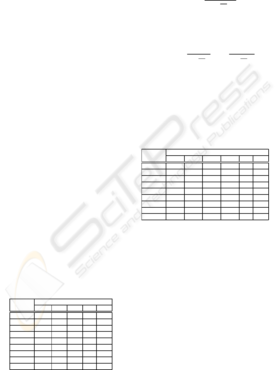
Step 1: Initialization

The construction of the tree starts with the selection of

the Start node as the tree root. This node is identiﬁed

by the number zero. Figure 2 shows the contents of

node zero.

Start

UB:943

LB:357

Insertion order

Upper bound

Lower bound

Software tool

Values in thousands

of USA dollars

Start

UB:943

LB:357

Start

UB:943

LB:357

Start

UB:943

LB:357

Insertion order

Upper bound

Lower bound

Software tool

Values in thousands

of USA dollars

Figure 2: The contents of node zero.

Note that the upper bound of node zero is the sum

of two values. The ﬁrst, is the sum of the NPV of each

software unit (MMF or AE) belonging to the currently

known part of the development sequence of software

units. The second is the sum of the maximum NPV of

each unit belonging to the unknown part.

Because node zero is the only one in the tree, its

upper bound is the sum of the highest NPV of each

software unit throughout the whole project’s window

of opportunity, considering the precedence restric-

tions introduced in Figure 1. Therefore, the upper

bound of node zero, i.e. ub(0), is given by

ub(0) = npv(GIL, 9) + npv(PdS, 2)+ npv(PsS, 4)+

npv(Pc, 3) + npv(CD, 4) + npv(LP, 5)+

npv(SC, 5) + npv(CP, 6) + npv(CLM, 9)

= −42+ 134+ 157+ 87+ 71+ 11+ 53+

30+ 441

= $943

It should be noted that in formula the highest NPV

of unit Pc throughout the window of opportunity is

$87, and not $115 as one could expect. This happens

because the precedence restrictions introduced in Fig-

ure 1 do not allow Pc to be developed until the third

period.

The lower bound of node zero is the sum of the

lowest NPV of each software unit throughout the win-

dow of opportunity from the earliest period in which

each unit may be developed, considering the prece-

dence restrictions introduced in Figure 1. Therefore,

lb(0) = vpl(GIL, 1) + vpl(PdS, 9) +vpl(PsS, 9)+

vpl(Pc, 9) + vpl(CD, 9) + vpl(LP, 9)+

vpl(SC, 9) + vpl(CP, 9) + vpl(CLM, 9)

= −49+ 15+ 31+ 11− 10− 5− 71−

6+ 441

= $357

Observe that, in the worst case, to calculate both

the upper and lower of a node one has to visit all el-

ements of Table 3. Therefore, these value can always

be obtained in a polynomial time.

Step 2: Doing the initial branch

The search for the sequence of software units that

maximizes the project’s NPV goes on with the inser-

tion, in the search tree, of the nodes that corresponds

to the units that may be developed in the next period.

In this case, the choice is obvious, given that node

zero is the only node in the tree and GIL is the only

tool that may be developed immediately after. Figure

3 shows the search tree after the insertion of node 1,

corresponding to the GIL unit. The calculation of its

upper and lower bounds are done as described in Step

Step 6: Selecting a node to branch

The search goes on according to the steps already de-

scribed until the tree reaches the state presented in

Figure 4 and a decision must be made: which node

should be branched?

At this point, several possibilities are available.

For example, one may choose the node with the high-

est upper bound, the one with highest lower bound,

or even the one with the highest average between its

ICEIS 2008 - International Conference on Enterprise Information Systems

166

1 GIL

UB:935

LB:357

1 GIL

UB:935

LB:357

1 GIL

UB:935

LB:357

Start

UB:943

LB:357

Start

UB:943

LB:357

Start

UB:943

LB:357

Figure 3: The contents of node one.

lower and upper bound. In the absence of hard evi-

dence on which criteria is the best, a heuristic has to

be established. In this case, throughout the building of

the whole search tree, the algorithm always opt for the

node with the highest upper bound. Therefore, node

4 is selected for branching.

1 GIL

UB:935

LB:357

1 GIL

UB:935

LB:357

1 GIL

UB:935

LB:357

2 PdS

UB:935

LB:476

2 PdS

UB:935

LB:476

2 PdS

UB:935

LB:476

3 Pc

UB:935

LB:552

3 Pc

UB:935

LB:552

3 Pc

UB:935

LB:552

5 CD

UB:873

LB:633

5 CD

UB:873

LB:633

5 CD

UB:873

LB:633

4 PsS

UB:919

LB:678

4 PsS

UB:919

LB:678

4 PsS

UB:919

LB:678

Start

UB:943

LB:357

Start

UB:943

LB:357

Start

UB:943

LB:357

Figure 4: Search tree when node 4 is selected for branching.

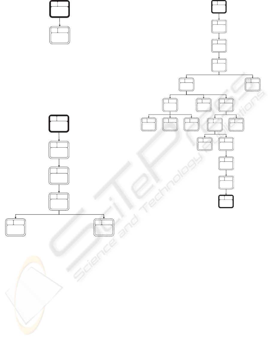
Step 13: Identifying the optimal solution

The search proceeds until the tree achieves the state

described in Figure 5.

At this point, there is no node that has an upper

bound that is higher than the lower bound of node

18, which cannot be branched. Therefore, the search

stops, and the path to node 18 corresponds to the

sequence that maximizes the NPV of the software

project, i.e. Start → GIL → PdS → Pc → PsS →

SC → CD → CP → LP → CLM → End, which yields

an NPV of $878.

It is important to observe that many nodes are

not branched during the search process. For exam-

ple, node 5 is never branched. This happens for two

reasons. First, while being considered for branching,

its upper bound is never the highest. Second, when

node 15 is inserted into the tree, the upper bound of

1 GIL

UB:935

LB:357

1 GIL

UB:935

LB:357

1 GIL

UB:935

LB:357

2 PdS

UB:935

LB:476

2 PdS

UB:935

LB:476

2 PdS

UB:935

LB:476

3 Pc

UB:935

LB:552

3 Pc

UB:935

LB:552

3 Pc

UB:935

LB:552

5 CD

UB:873

LB:633

5 CD

UB:873

LB:633

5 CD

UB:873

LB:633

4 PsS

UB:919

LB:678

4 PsS

UB:919

LB:678

4 PsS

UB:919

LB:678

6 CD

UB:882

LB:743

6 CD

UB:882

LB:743

6 CD

UB:882

LB:743

8 SC

UB:886

LB:803

8 SC

UB:886

LB:803

8 SC

UB:886

LB:803

7 LP

UB:858

LB:694

7 LP

UB:858

LB:694

7 LP

UB:858

LB:694

13 CP

UB:847

LB:778

13 CP

UB:847

LB:778

13 CP

UB:847

LB:778

12 SC

UB:866

LB:835

12 SC

UB:866

LB:835

12 SC

UB:866

LB:835

11 LP

UB:839

LB:754

11 LP

UB:839

LB:754

11 LP

UB:839

LB:754

9 CD

UB:882

LB:850

9 CD

UB:882

LB:850

9 CD

UB:882

LB:850

10 LP

UB:858

LB:814

10 LP

UB:858

LB:814

10 LP

UB:858

LB:814

15 CP

UB:878

LB:874

15 CP

UB:878

LB:874

15 CP

UB:878

LB:874

14 LP

UB:870

LB:858

14 LP

UB:870

LB:858

14 LP

UB:870

LB:858

16 LP

UB:878

LB:878

16 LP

UB:878

LB:878

16 LP

UB:878

LB:878

17 CLM

UB:878

LB:878

17 CLM

UB:878

LB:878

17 CLM

UB:878

LB:878

Start

UB:943

LB:357

Start

UB:943

LB:357

Start

UB:943

LB:357

End

UB:878

LB:878

End

UB:878

LB:878

End

UB:878

LB:878

Figure 5: The search tree generated by the branch & bound

method.

node 5 (which is the highest value that a sequence

of units that starts with GIL → PdS → Pc → CD may

have)is lower than the lowerbound of node 15 (which

is the lowest value that a sequence that starts with

GIL → Pds → Pc → PsS → SC → CD → CP may re-

turn). As a result, node 5 ceases to be considered for

branching.

4 THE BRANCH & BOUND

ALGORITHM

In formal terms , the branch & bound algorithm that

maximizes the NPV of a software project is described

as follows. Given

• A precedence graph of software units G(V

, E

composed of a set of software units V

, and the

precedence restrictions described in E

;

• A window of opportunity P and

MAXIMIZING THE BUSINESS VALUE OF SOFTWARE PROJECTS - A Branch & Bound Approach

167

• A discount rate r.

The sequence S of software units v

∈ V

that yield

the highest NPV is found by the following algorithm:

Ω

← {Start}; Θ

←

0; Q ← {Start};

Repeat :

N ← q ∈ Q, such that ub(q) =

Maximum({ub(q

′

)|q

′

∈ Q}),

Ω

← Ω

∪ eligible(N),

← Θ

∪ {(N, e)|e ∈ eligible(N)},

MaxLB ← Maximum({lb(v)|v ∈ Ω

}),

Q ← {v ∈ Ω

|v ∈ (Q− {N}) ∪ eligible(N) ∧

ub(v) ≥ MaxLB},

Until Q =

S ← path to(N).

where:

• S is the best solution among the nodes in Q;

• Ω

is the set of nodes in the search tree;

• Θ

is the set of edges connecting search tree

nodes;

• MaxLB is the highest lower bound so far; and

• Q is the list of candidate nodes.

4.1 The Upper Bound Heuristic

The upper-bound function ub(n ∈ Ω

) → R returns

the maximum NPV that a development sequence of

software units may yield considering the known part

of the sequence, i.e. the sequence that goes from the

tree root to node n.

ub(n) ←

∑

npv(s

, i) such that s

∈ path to(n)+

∑

npvMax(v

, when(n, v

)) such that

∈ (V

− {v

∈ path to(n)})

4.2 The Lower Bound Heuristic

The lower bound function lb(n ∈ Ω

) → R returns

the minimum NPV that a development sequence of

software units may yield considering the known part

of the sequence, i.e. the sequence that goes from the

tree root to node n.

lb(N) ←

∑

npv(s

, i) such that s

∈ path to(n)+

∑

npvMin(v

, when(n, v

)) such that

∈ (V

− {v

∈ path to(n)})

4.3 Auxiliaries Functions

The branch & bound method also make use of the fol-

lowing functions:

• eligible(N ∈ Ω

) → PV

that returns the set of

possible immediate successors of a node n in the

search tree.

• path to(N ∈ Ω

) → SeqV

that returns the se-

quence of software units that leads to the node N

of the search tree.

• when(v

∈ V

, n ∈ Ω

) → P that returns the earli-

est period in which a software unit v

may be de-

veloped, considering the sequence that goes from

the tree root to n.

5 DISCUSSION

At the outset of this article the authors undertook to

successfully present a branch & bound approach that

allows managers to determine the optimum order for

the development of a network of software units. Bel-

low we answer some key questions about the implica-

tions of the method to software development and the

deployment of business strategy.

5.1 Why should a Branch & Bound

Method be used to Maximize the

NPV of a Software Project?

The number of possible development sequences of

a network of software units tends to grow exponen-

tially according to the number of MMFs and AEs into

which a software project is divided, making it difﬁcult

to ﬁnd their optimum implementation order in a fea-

sible time. Consequently, the search for the optimum

order beneﬁts from the use of heuristic methods such

as the branch & bound that, in most cases, does not

need to enumerate all possible sequences of software

units to indicate the optimum (Liberti, 2003).

5.2 What does this Method offer that

the IFM does not?

There are two major advantages in using the branch

& bound method instead of the IFM. The ﬁrst is that

it ensures that an optimal solution to a problem is al-

ways found, while the IFM may provide inferior re-

sults with no warning. In projects that cost millions of

US dollars, even a small difference from the optimal

solution may lead to a loss of a substantial amount

of money. Losses of this magnitude may hamper

business competitiveness,allowing the growthof rival

companies. The second advantage is that this method

can be applied to projects that present multiple depen-

dencies among its software units, which is frequently

the case in real-world software projects.

ICEIS 2008 - International Conference on Enterprise Information Systems

168

5.3 Does the Branch & Bound Method

allow for Parallel Development?

No, it does not. Actually, building a branch & bound

algorithms that deals with the parallel development

of MMFs and AEs is still an open problem. How-

ever, the vast majority of software projects in the real

world are run by small companies that do not have the

personnel nor the necessary resources to use parallel

development (Harris et al., 2007).

5.4 What is the Expected Effect of the

Branch & Bound Method on

Software Development?

Because of the tough competition that are currently

being experienced in many different markets, nowa-

days many companies are offshoring the development

of software, creating a healthy competitive environ-

ment in which software companies compete against

each other for contracts. Obviously, proposals that

maximize the ﬁnancial value of a software project

provide a better competitive position in regard to

those that have adopted a more traditional view of the

software development.

Moreover, it is important to keep in mind that the

smaller investment in the development of a software

project provided by the branch & bound method fa-

vors the development of other projects that could not

be executed otherwise. All of this, favor the existence

of companies that are more efﬁcient and better pre-

pared to compete in the world market.

6 CONCLUSIONS

This article presented a branch & bound method that

identiﬁes the development plan that maximizes the

business value of a software project. The method al-

ways ﬁnds the best solution and does not imposes un-

reasonable limitations to the precedence relations that

may exist among the software units, facilitating the

development of complex software projects from a rel-

atively small investment.

REFERENCES

Abacus, A., Barker, M., and Freedman, P. (2005). Us-

ing test-driven software development tools. Software,

IEEE, 22(2):88–91.

Denne, M. and Cleland-Huang, J. (2004a). The incremental

funding method: data-driven software development.

IEEE Software, 21(3):39–47.

Denne, M. and Cleland-Huang, J. (2004b). Software

by Numbers - Low-Risk, High-Return Development.

Prentice Hall.

Denne, M. and Cleland-Huang, J. (2005). Financially in-

formed requirements prioritization. In Roman, G.-C.,

Griswold, W., and Nuseibeh, B., editors, 27

inter-

national conference on Software Engineering, pages

710–711, St. Louis, MO, USA. ACM.

Fabozzi, F. J., Davis, H. A., and Choudhry, M. (2006). In-

troduction to Structured Finance. John Wiley.

Gross, J. L. and Yellen, J. (2005). Graph Theory and Its

Applications. Chapman & Hall and CRC, 2

edition.

Harris, M., Aebischer, K., and Klaus, T. (2007). The

whitewater process: Software product development in

small IT businesses. Communications of the ACM,

50(5):89–93.

Helo, P., Hilmola, O.-P., and Maunuksela, A. (2004). Man-

aging the productivity of product development: a sys-

tem dynamics analysis. International Journal of Man-

agement and Enterprise Development, 1(4):333–344.

Highsmith, J. (2002). Agile Software Development Ecosys-

tems. Addison-Wesley.

Hillier, F. S. and Lieberman, G. J. (2001). Introduction to

operations research. McGraw-Hill, New York, NY,

edition.

Hubbard, D. W. (2007). How to Measure Anything: Finding

the Value of “Intangibles” in Business. John Wiley.

Jorgenson, D. W., Ho, M. S., and Stiroh, K. J. (2003).

Growth of us industries and investments in informa-

tion technology and higher education. Economic Sys-

tems Research, 15(3):279–325.

Lam, H. (2004). New design-to-test software strategies ac-

celerate time-to-market. In 29

International Elec-

tronics Manufacturing Technology Symposium, pages

140–143, San Jose, CA, USA. IEEE.

Liberti, L. (2003). Optimization and Optimal Control, chap-

ter Comparison of Convex Relaxations for Monomials

of Odd Degree, pages 165–174. Computers and Op-

erations Research. World Scientiﬁc.

McManus, J. C. (2003). Risk Management in Software De-

velopment Projects. Elsevier.

Nord, R. and Tomayko, J. (2006). Software architecture-

centric methods and agile development. Software,

IEEE, 23(2):47–53.

Rashid, A., Moreira, A., and Ara´ujo, J. (2003). Modu-

larisation and composition of aspectual requirements.

In Proceedings of the 2

International Conference

on Aspect-oriented Software Development, pages 11

– 20, Boston, Massachusetts, USA. ACM.

Steindl, C. (2005). From agile software development to

agile businesses. In Matos, J. S. and Crnkovic, I.,

editors, 31

EUROMICRO Conference on Software

Engineering and Advanced Applications, pages 258–

265, Porto, Portugal. Porto University.

Whittle, R. and Myrick, C. B. (2005). Enterprise Business

Architecture. Auerbach.

MAXIMIZING THE BUSINESS VALUE OF SOFTWARE PROJECTS - A Branch & Bound Approach

169