OPTIMAL LAYOUT SELECTION USING PETRI NET IN AN

AUTOMATED ASSEMBLING SHOP

Iraj Mahdavi

, Mohammad Mahdi Paydar

, Babak Shirazi

and Magsud Solimanpur

Department of Industrial Engineering, Mazandaran University of Science & Technology, Babol, Iran

Urmia University, Urmia, Iran

Keywords: Petri net, Automated assembling shop, Production cycle time, WIP.

Abstract: Abstract In today's competitive manufacturing systems, it is crucial to respond quickly to the demand of

customers and to decrease total cost of production. To achieve higher performance of automated assembling

shop, it is needed to utilize methods to minimize production cycle time (makespan) and work-in-process

(WIP) in buffers. This paper intends to focus on the selection of optimal layout based on allocation of

machines to different locations as they can perform similar operations with different processing times. The

time Petri net (TPN) has been used to illustrate the applications of proposed model in case study.

1 INTRODUCTION

Layout designing have been extensively researched

in many manufacturing systems. Researches have

mainly concentrated on the important class of

systems called flow shops, in which components are

moved linearly through the system, and

manufacturing stations are totally dedicated (Adel

and Baz, 2004). Now a days, automatic tools such as

computer numerical control (CNC) machines and

different types of robots have been used in assembly

lines called automated assembling shop. Automated

assembling shop consists of several types of CNC

machines, robots, and automated guided vehicles

designed to produce a great variety of products in

multiple lines. Many products can be manufactured

and assembled in automated assembling shop. The

parts to be assembled are transferred by conveyors

and robots. Robots transfer the parts from the

conveyors to buffer. The main problem of designing

an automated assembling shop is to obtain the

minimum production cycle time and WIP (Hsieh et

al, 2007).

In the literature, this problem is most often

treated as a single objective problem and only the

capacity constraints of the assembly shop are

considered. For example, Boubekri and Nagaraj

(1993) developed an integrated approach for the

selection and design of assembly systems. A model

for evolutionary implementation of efficient

assembly systems was proposed by Rampersad

(1994, 1995). But very little has been reported on

the design of assembly systems and system layout.

Due to the discrete nature, Petri nets (PN) are

widely used for modeling manufacturing systems

(Park et al., 2001, Yan et al., 2003). Petri net is a

graphical and mathematical modeling tool for

describing and studying systems (Jehng, 2002). In

the early development of Petri nets (Petri, 1962) and

(Peterson, 1981), it was particularly concerned with

the description of the causal relationships between

events. Much of the early theory, notation, and

representation of Petri nets have been developed for

discrete event systems. (Ramchandani, 1974)

showed how Petri nets could be applied to the

modeling and analysis of systems of concurrent

components. There have been reports of Petri nets

applications in the representation, analysis and

control of flexible assembling system/ flexible

manufacturing system (Alla et al., 1984), (Cecil et

al., 1992), (Muro-Medrano et al., 1992), and

(Moore, 1996). Petri nets have been used to model

robotic or assembly processes so that a sequence of

operations is generated based on the Petri net model.

On the other hand, many attempts have also been

made to extend and modify conventional Petri nets

to enhance their modeling power for assembly

systems. This resulted in net variations such as

colored Petri nets, control nets, timed Petri nets, and

object Petri nets. This paper focuses on the layout

519

Mahdavi I., Mahdi Paydar M., Shirazi B. and Solimanpur M. (2008).

OPTIMAL LAYOUT SELECTION USING PETRI NET IN AN AUTOMATED ASSEMBLING SHOP.

In Proceedings of the Tenth International Conference on Enterprise Information Systems - AIDSS, pages 519-523

DOI: 10.5220/0001703905190523

 SciTePress

designing in automated assembling shops. Since

some machines can perform different operations in

different processing times, the machines are

allocated to different locations so that the total

production cycle time and WIP are minimized.

2 PETRI NET MODELING

A timed-PN is able to describe a time dependent

system. Two methods exist to model timing: either

timing associated with places (the PN is said to be

place-timed Petri net, or P-timed PN), or timing

associated with transitions (the PN is said to be

transition-timed Petri net, or T-timed PN). It also

can be shown that P-timed PNs and T-timed PNs are

equivalent, and it is possible to move from one

model to the another (Zhang et al., 2005).

This paper addresses a production system that

receives an order from customers. According to the

order, an initial layout and machine allocation of

production line is designed. The automated

assembling shop for this model consists of two

conveyor robots (R

, R

). There are nine machines

(M1, M2,..., M9), five work pieces (A, B, C, D, E)

and fourteen operations (OP

,..., OP

). We

consider five buffers in the layout such that their

amount of WIP is different. Figure 1 is a graphical

representation of material flow in the manufacturing

system based on the above information. The

machines M

, M

and M

can perform either of

operations OP

, OP

and OP

in different

processing times. The problem is to find the

optimum allocation of these machines for doing

these operations to minimize the total production

cycle time and WIP.

Figure 1: System configuration of automated assembeling

shop.

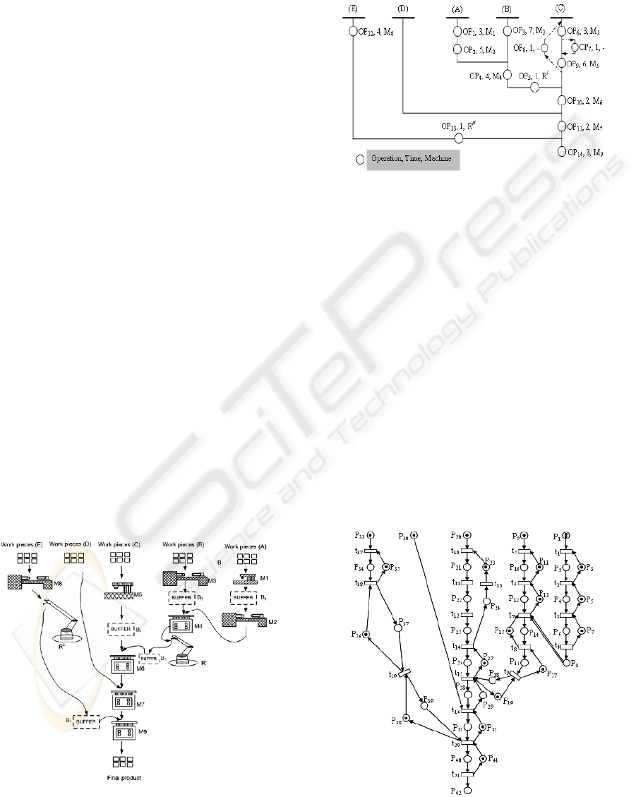
Figure 2 shows a specific allocation of these

machines in which operations OP

, OP

and OP

are performed by machines M

, M

and M

respectively.

Figure 2: The OPC of automated assembling shop.

In Figure 2, the Operation Process Chart (OPC) of

the manufacturing system is shown. The OPC is

used for showing the procedure through which work

pieces are assembled and all operations in the

process of manufacturing system. In OPC,

purchased work piece (work piece D) is connected

to the basic line (work piece C) by a horizontal line.

The operations that are connected to the basic line

by dash line (OP

) represent tool changing in

machine M

2.1 P-timed PN Model of Automated

Assembling Shop

For the PN model of automated assembling shop

shown in Figure 3. Place-timed Petri nets (P-timed

PN) are used to model the system, in which

transitions represent events and the places represent

states, or conditions.

Figure 3: The PN model of automated assembling shop.

ICEIS 2008 - International Conference on Enterprise Information Systems

520

The role of transitions and places in the proposed

PN model are shown in Tables 1 and 2, respectivly.

Table 1: Role of transitions in the proposed PN model.

Transitions

: Operation OP

starts

: Operation OP

finishes

: Operation OP

starts

: Operation OP

finishes

: Operation OP

starts

: Operation OP

finishes

: Operation OP

starts

: Operation OP

finishes& Operation OP

starts

: Operation OP

finishes

: Operation OP

starts

: Operation OP

finishes& Operation OP

starts

: Operation OP

finishes& Operation OP

starts

: Operation OP

finishes

: Operation OP

finishes& Operation OP

starts

: Operation OP

starts

: Operation OP

finishes & Operation OP

starts

: Operation OP

starts

: Operation OP

finishes& Operation OP

starts

: Operation OP

finishes

: Operation OP

finishes& Operation OP

starts

: Operation OP

finishes

Table 2: Role of places in the proposed PN model.

Places

: Work piece A available

: Operation OP

: Machine M1 available

: Work piece A ready for the operation OP

: Buffer of work piece A available

: Operation OP

: Machine M2 available

: Work pieces A available to assemble

: Work piece B available

: Operation OP

: Machine M3 available

: Work piece A ready for the operation OP

: Buffer of work piece B available

: Operation OP

: Machine M4 available

: Operation OP

: Robot R

available

: Work piece B ready for the assemble

: Buffer of work piece B available

: Work piece C available

: Operation OP

: Machine M5 available

: Operation OP

: Work piece C ready for the operation OP

: Buffer of work piece C available

: Operation OP

Table 2: Role of places in the proposed PN model(cont).

Places

: Machine M6 available

: Work piece D available

: Operation OP

: Machine M7 available

: Work piece E available

: Operation OP

: Machine M8 available

: Robot R

available

: Operation OP

: Buffer of work piece E available

: Work piece E ready for to assemble

: Operation OP

: Machine M9 available

: Final product available

3 PROPOSED METHOD TO

SELECT OPTIMAL LAYOUT

The production cycle time is obtained by MATLAB

Petri net toolbox. The maximum WIP (WIP

max

) is

calculated according to the maximum number of

tokens in buffer places (p

, p

). The

average work-in-process (WIP

average

) for each buffer

can be obtained as discussed below.

We define the following notation:

i : is the number of work pieces

()

1, 2,....,iN=

j : is the number of buffers

()

1, 2,....,jM=

t : is the discrete unit time

()

1, 2....,tT=

k : is the number of allocations

()

1, 2,...,kL=

Decision Variable:

1 If work piece is in buffer at time

0Otherwise

ijt

⎧

⎨

⎩

According to the notations, we obtain the WIP

average

of j

buffer for each state as given in equation (1).

()

ijt

average

WIP WIP

∑∑

(1)

We calculate the average WIP of buffer j among all

the allocations as given in equation (2).

(

)

111

Average W IP within all allocations WIP

LNT

ijt

kit

===

⎛⎞

⎜⎟

⎝⎠

⎜⎟

⎝⎠

∑∑∑

(2)

OPTIMAL LAYOUT SELECTION USING PETRI NET IN AN AUTOMATED ASSEMBLING SHOP

521

For allocation k, we calculate the value

()

as a

decision criterion for selection of optimum

allocation as given in equation (3).

()

(

)

zxy

FFF=+ : (3)

where

()

(

)

111

LNT

ijt

kit

it k

FCWIPWIP

TTL

===

⎛⎞

=−=

⎜⎟

⎝⎠

⎛⎞

⎜⎟

⎝⎠

⎜⎟

−

⎜⎟

⎝⎠

∑

∑∑∑

∑∑

∑

()

minyTk

FCTT=−

: is the cost coefficient of buffer j.

: is the cost coefficient of production cycle time.

∑

: is the makespan of allocation k.

min

T : is the minimum makespan among all the

allocations.

Finally, the allocation with minimum

is selected.

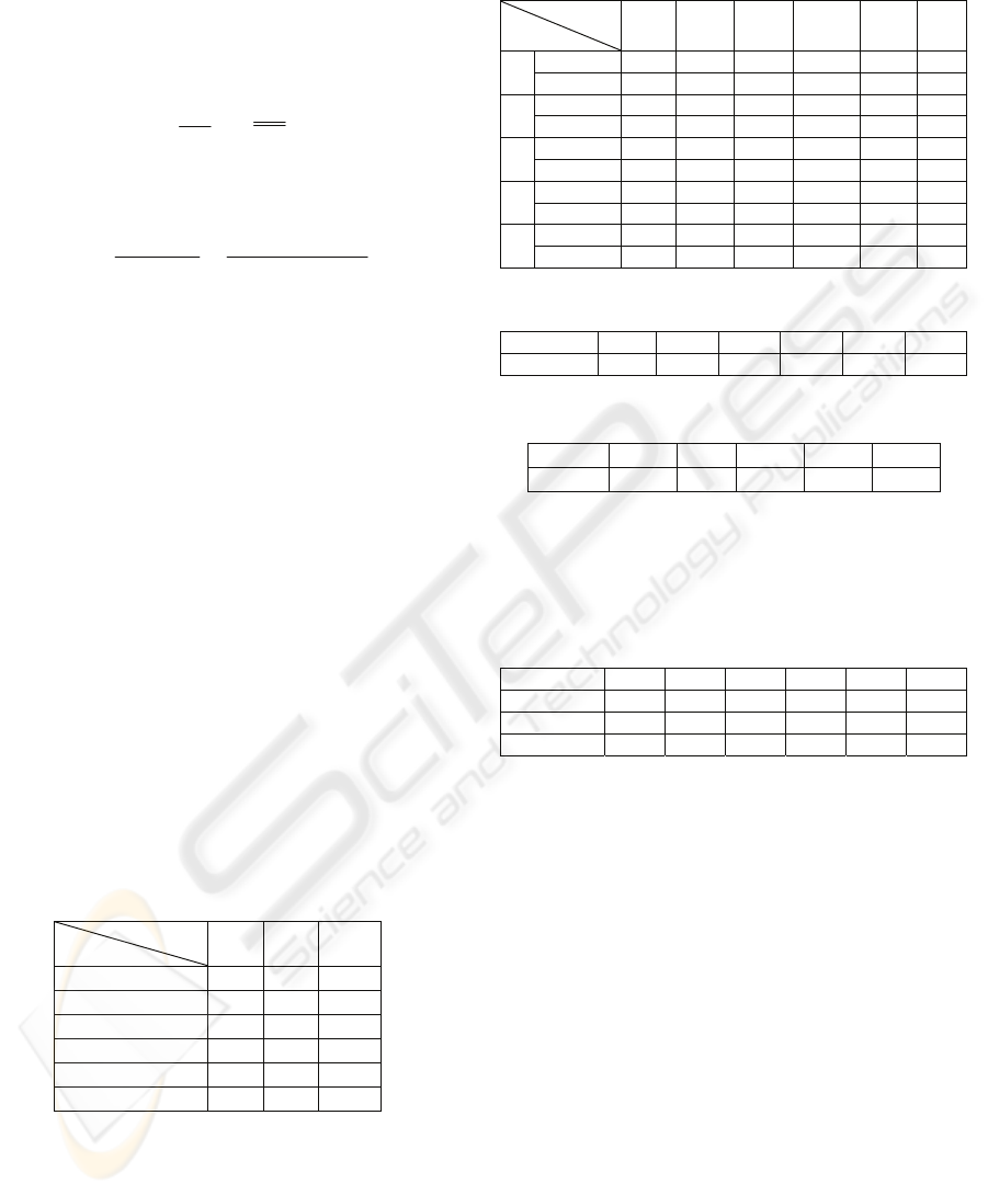
4 COMPUTATIONAL RESULTS

Assume that ten products are to be produced in the

manufacturing system discussed above. Table 3

shows six possible allocations of machines M

, M

and M

for doing operations OP

, OP

and OP

Table 3: Possible allocations of machines M

, M

and M

for operations OP

, OP

and OP

Operation

Allocation

1 M

2 M

3 M

4 M

5 M

6 M

The simulation results of WIP in each buffer and the

production cycle time of each allocation have been

given in Tables 4 and 5, respectively.

As a managerial consideration, let us assume that

the cost coefficient value of production cycle time is

0.4, i.e. C

= 0.4, and the cost coefficient value of

each buffer is as shown in Table 6.

Table 4: The average and maximum WIP of each buffer in

different allocations.

Allocation

Buffe

1 2 3 4 5 6

WIP

ave

4.8 4.8 3.3 3.3 1.6 1.6

WIP

max

11 11 8 8 5 5

WIP

ave

3.4 3.7 3.1 1.7 1.7 0.7

WIP

max

7 8 7 4 5 2

WIP

ave

0 0 0.01 0.01 0.7 0.7

WIP

max

0 0 1 1 2 2

WIP

ave

1.6 1.6 0.3 0.3 0.1 0.8

WIP

max

3 3 1 1 1 1

WIP

ave

4.3 3.8 2.4 3.8 2.1 3.1

WIP

max

8 8 5 8 4 6

Table 5: The production cycle time of each allocation.

Allocation 1 2 3 4 5 6

Cycle time 155 155 116 116 116 116

Table 6: Cost coefficient value of each buffer.

Based on the computational results, the values of

functions

, F

and F

of each allocation are shown

in Table 7.

Table 7: The values of functions F

, F

and F

of each

allocation.

Allocation 1 2 3 4 5 6

)

0.64 0.67 0.12 0.14 0.29 0.41

)

15.6 15.6 0 0 0 0

)

16.2 16.3 0.12 0.1 0.29 0.41

As seen in Table 7, the allocation 3 has resulted in

minimum

and therefore this layout is selected as

the optimum allocation of machines.

5 CONCLUSIONS

In this paper, the allocation of machines for doing

different operations in an automated assembling

shop has been discussed. The system features

identical multi-functional machines with different

processing times. A P-timed PN is applied for

modeling of the manufacturing system. The

proposed model is able to determine the average and

maximum WIP in different buffers as well as the

production cycle time associated with each

allocation pattern. The optimal layout is obtained

based on minimum WIP

average

and production cycle

time.

Buffer

0.08 0.1 0.16 0.21 0.05

ICEIS 2008 - International Conference on Enterprise Information Systems

522

REFERENCES

Adel, M., Baz, E.l., 2004. A genetic algorithm for facility

layout problems of different manufacturing

environments. Computers & Industrial Engineering,

(47)2-3, 233-246.

Alla, H., Ladet. P., Martinez, J., 1984. Silva SM.

Modeling and validation of complex systems by

colored Petri nets application to a flexible

manufacturing system. In: Rozenberg G, editor.

Advances in Petri Net, Lecture Notes in Computer

Science, Vol. 188. NY: Springer, 15–31.

Boubekri, N., Nagaraj, S., 1993. An integrated approach

for the selection and design of assembly systems.

Integrated Manuf Systems, 4(1), 11–7.

Cecil, J.A., Srihari, K., Emerson, C.R., 1992. A review of

Petri net applications in manufacturing. Int J Adv

Manuf Technol, 7,168–77.

Hsieh, Y.J., Chang, S. E., Chang, S.C., 2007. Design and

storage cycle time analysis for the automated storage

system with a conveyor and a rotary rack. Inter-

national Journal Production Research, January (2007).

Jehng, W.K., 2002. Petri net models applied to analyze

automatic sequential pressing system. Materials

Processing Technology, 120, 115-125.

Moore, K.E., Gupta, S.M., 1996. Petri net models of

flexible and automated manufacturing systems: a

survey. Int J Prod Res, 34(11), 3001–35.

Muro-Medrano, P.R., Joaquin, E., Jose, L.V., 1992. A

rule-Petri net integrated approach for modeling and

analysis of manufacturing systems, In: Gentina JC,

Tzafestas SG. Editors, Robotics and flexible

manufacturing systems, Amsterdam: Elsevier Science

Publishers (North-Holland), 349–58.

Park, E., Tilbury, D.M., Khargonekar, P.P., 2001. A

modeling and analysis methodology for modular logic

controllers of machining systems using Petri net, IEEE

Trans Robotics Automat, 5(2), 168–88.

Peterson, J.L., 1981. Petri Net Theory and the Modeling of

Systems. Prentice-hall, Englewood Cliffs, NJ.

Petri, C., 1962. Kommunikation Mit Automation. Thesis

(Ph.D), Dissertation University of Bonn, Bonn, West

Germany.

Ramchandani, C., 1974. Analysis of Asynchronous

Concurrent System by timed Petri nets, Doctoral

Dissertation, NIT, Cambridge, NA.

Rampersad, H.K., 1994. Integrated and simultaneous

design for robotic assembly. New York, Wiley.

Rampersad, H.K., 1995. A case studies in the design of

flexible assembly systems. Int J Flexible Manuf

Systems, 7(3), 255–86.

Yan, H.S., Wang, Z., Jiao, X.C., 2003. Modeling,

scheduling and simulation of product development

process by extended stochastic high-level evaluation

Petri nets. Robotics Comput Integr Manuf, 19, 329–42.

Zhang, W., Freiheit, T., Yang, H., 2005. Dynamic

scheduling in flexible assembly system based on

timed Petri nets model, Robotics and Computer-

Integrated Manufacturing, 550-558.

OPTIMAL LAYOUT SELECTION USING PETRI NET IN AN AUTOMATED ASSEMBLING SHOP

523