PREDICTING THE ARRIVAL OF EMERGENT PATIENT
BY AFFINITY SET
Yuh-Wen Chen
Institute of Industrial Engineering and Technology Management, Da-Yeh University
112 Shan-Jeau Rd., Da-Tsuen, Chang-Hwa 51505, Taiwan
Moussa Larbani
Dpet. of Business Administration, Faculty of Economics, IIUM University, Jalan Gombak, 53100, Kuala Lumpur, Malaysia
Chao-Wen Chen
Department of Trauma, Hospital of Kaohsiung Medical University
100 Shi-Chuan 1st Rd., San Ming District, Kaohsiung City, Taiwan
Keywords: Patient Flow, Prediction, Affinity Set, Neural Network.
Abstract: Predicting the time series of emergent patient arrival is valuable in monitoring/tracking the daily patient
flow because these efforts keep doctors alarmed in advance. A prediction problem of the time series
generated by actual arrival of emergent patient is considered here. Traditionally, such a problem is analyzed
by moving average method, regression method, exponential smoothing method or some existed
evolutionary methods. However, we propose a new affinity model to accomplish this goal. Our data of time
series is actually recorded from hour to hour (hourly data) for three days: the data of the first two days are
used to generate/train prediction model; after that, the data of the final/third day is used to test our prediction
results. Two types of model: affinity model and neural network model are used for comparing their
performances. Interestingly, the affinity model performs better prediction results. This hints there could be a
special pattern within the time series generated by actual arrival of emergent patient.
1 INTRODUCTION
In many medical domains the doctors need to learn
why a decision was made, otherwise they are
unlikely to trust the advice generated by automated
data analysis methods. Data mining/knowledge
discovery can solve such problems (Abdel-Aal and
Al-Garni, 1997). Important requirements for
knowledge discovery are interpretability, novelty,
and usefulness of the results. Many data mining
problems involve temporal aspects. The most
common form of temporal data is time series where
some properties are repeatedly observed generating
a series of data items similar in structure: we define
this similarity as a special pattern sometime.
However, the pattern could be very dynamic and
complicated in reality (Agrawal and Srikant, 1995).
Correctly tracking, monitoring and predicting the
arrival of emergent patient in hospital are important
and crucial to the clinical operation of hospital
(TeleTracking, 2006). Because such efforts will help
doctors realize what the level of service (LOS) for
patients is, then they can appropriately response in
advance by these data. In addition, these efforts are
able to avoid system breakdown of hospital because
of too many patients. There could be many ways of
predicting time series, for example, moving average
method, regression method, exponential smoothing
method, or other evolutionary techniques. In this
study, we show the innovative thinking to predict
time series, this goal is achieved by affinity set
(Larbani and Chen, 2006). Affinity is defined by two
types (Larbani and Chen, 2006): the first type is
natural liking for or attraction to a person, thing,
idea, etc. For example, friendship is a kind of direct
affinity. In order to take place, such affinity requires
the subjects between whom the affinity takes place
and the affinity itself. The second type is defined as
273
Chen Y., Larbani M. and Chen C. (2008).
PREDICTING THE ARRIVAL OF EMERGENT PATIENT BY AFFINITY SET.
In Proceedings of the Tenth International Conference on Enterprise Information Systems, pages 273-277
DOI: 10.5220/0001723402730277
Copyright
c
 SciTePress

a close relationship between people or things that
have similar qualities, structures, properties,
appearances or features. In this paper we call it
indirect affinity. Simply speaking, affinity represents
the closeness/distances between any two objects. We
only use the direct affinity modelling to predict the
time series generated by actual arrival of emergent
patient, and the performance of affinity model is
compared with that of neural network (NN) model
(Kim and Han, 2000). Interestingly, the errors of
affinity model are smaller than those of the NN
model. Thus, exploring and developing affinity
models are valuable in the very near future.
This paper is organized as follows: in Section 2, we
show the technical background for this study,
including the necessary affinity definitions. In
Section 3, an actual example of emergent patient
arrival is presented. Two types of models: NN model
and affinity model are both used to predict the time
series; furthermore, their performances are
compared. Finally, conclusions and
recommendations are in Section 4.
2 TECHNICAL BACKGROUND
In this section, we will simply review two prediction
models: affinity model and NN model.
2.1 Basic Concepts of Affinity
Here, the basic definitions are shortly reviewed
(Larbani and Chen, 2006).
Definition 2.1. Affinity Function.
Let e be an object and A be an affinity set,
respectively. The affinity between e and A is
represented by a function that we call affinity
function.
e
A
M ( . ): [0,+
∞
] → [0,1]
t
→
e
A
M (t)
The value
e
A
M (t) expresses the degree or
strength of the affinity between object e the affinity
set A at time t. When
e
A
M (t) = 1 this means that the
object e satisfies completely the affinity that
characterizes A. When
e
A
M (t) = 0 this means that e
doesn’t satisfy the affinity characterizing A at all at
times t. When 0 <
e
A
M (t) < 1, this means that e
satisfies partially the affinity characterizing A at
time t.
Definition 2.2. The Universal Affinity Set.
The universal affinity set, denoted by U, is the
affinity set defined by the fundamental principle of
existence, that is,
e
U
M (t)=1, for all existing objects
at time t, and for all times t, that is, past present and
future.
Often in real problems the complete affinity
satisfaction
e
A
M (t)=1 may not be reached in real-
world situations for a given affinity set A and an
object e.
Definition 2.3. k-t-Core of a Affinity Set.
Let A be an affinity set and
]1,0[∈k . We say that
an object/element e is in the k-t-core of the affinity
set A at time t, denoted by k-t-core(A), if
e
A
M (t) ≥
k, that is, the k-t-core of A at time t is the traditional
set k-t-core(A)=
{
}
kte
e
≥)(M|
A
. When k =1, the
1-t- core(A) is simply called the core of A at time t,
denoted by t-core(A). The content of an affinity set
can be defined at any time by its membership
function. Let us give a formal definition of this
function. The k could be pre-decided or be viewed
as a decision value according to various problems.
Definition 2.4. Function Defining an Affinity Set.
Let A be a affinity set then the affinity defining A
can be characterized by the following function
R
A
(., .): U×[0, +∞] → [0,1] (1)
(e, t) → R
A
(e, t)=
e
A
M (t)
called affinity function.
In general, in real world situations, some
traditional referential set V, such that when an object
e is not in V,
e
A
M (t)=0 for all t, can be
determined, then the affinity defining A can be
defined by the following function
R
A
(., .): V×[0, +∞[→ [0,1]
(e, t) → R
A
(e, t)=
e
A
M (t)
We had larned earlier in Section 1 there are two
types of affinity : indirect affnity and direct affinity.
In this study, we only use the direct affinity for
modelling, which are briefly introduced as follows.
Definition 2.5. Let V and I be a referential set and a
subset of the time axis [0, +
∞ [ respectively. A time
dependent fuzzy relation R such that
(.)R
.) , (.
]1,0[V)(VI: →
×
×
(2)
)(R)),(,(
),(
tset
se
→
is called direct affinity on the referential V.
ICEIS 2008 - International Conference on Enterprise Information Systems
274

Interpretation 2.1. i) For any fixed time t the
relation (2) reduces to an ordinary fuzzy relation
)(R
.) , (.
t ]1,0[VV: →×
)(R),(
),(
tse
se
→
that expresses the intensity or the degree of affinity
between any couple of elements in V. Hence the
fuzziness of affinity between elements is taken into
account in Definition 2.5.
ii) For any fixed couple of elements
V),(
∈
se , the
relation (2) reduces to a fuzzy set defined on the
time-set I
(.)R
) , ( se
]1,0[I: →
)(R
),(
tt
se
→
that expresses the evolution over time of affinity
between the elements e and s.
Definition 2.6. Let R be a time-dependent fuzzy
relation defined on a subset of time axis I and a
referential V. Let A and B be two subsets of V. Then
the affinity between A and B can be described by the
following function
(.)R
)B ,A (
]1,0[I: → (3)
)(R
B)(A,
tt →
where
(.)R
B) ,(A
can be defined by many ways,
depending on the decision maker. For example,
)(R
B) ,(A
t
=
sese ≠×∈ ,BA),(
max
)(R
),(
t
se
, for all I
∈
t ,
or
)(R
B) ,(A
t =
sese ≠×∈ ,BA),(
min )(R
),(
t
se
, for all
I∈t (Larbani and Chen, 2006).
Here also for practical purpose we define the t-k-
affinity.
Definition 2.7. Let R be a time-dependent fuzzy
relation defined on a subset of time axis I and a
referential V. Let
]1,0[
∈
k
, and I∈t .
i) We say that a couple (e, s) has k affinity degree at
time t or it has t-k-affinity degree if
kt
se
≥)(R
),(
.
ii) A subset D of V has t-k-affinity degree if
ktR ≥)(
)DD,(
. Thus the t-k-affinity degree of
subsets depends on how is defined the affinity
between groups or subsets as indicated in Definition
2.6. In this study, k is regarded as a decision
variable, we want to find an affinity set that
maximizing k.
2.2 Neural Network Model
Since NN models are very popular and have
significant contributions in the data mining history,
we won’t duplicate the importance of NN so as to
save the paper length. Neural network models are
popularly used in many fields for prediction of time
series (Kim and Han, 2000; Kimoto and Asakawa,
1990). In addition, the NN models had already
achieved good prediction results. Therefore, in this
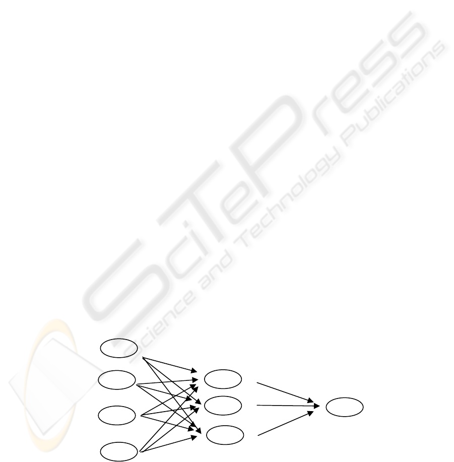
study, we introduce a simple NN model of time
series for prediction, this is shown in Fig. 1. This
model is designed as using the previously
fourobservations to reason the coming/fifth
observation.
3 PREDICTING THE ARRIVAL
OF EMERGENT PATIENT
In this section, we use two models: affinity model
and NN model to predict the arrival of emergent
Figure 1: Structure of NN Model.
D
t+1
D
t+2
D
t+3
D
t+4
Input Layer Hidden Layer
Output Layer
F
t+5
PREDICTING THE ARRIVAL OF EMERGENT PATIENT BY AFFINITY SET
275

patient simultaneously. Data of emergent patient
arrival for three days are actually collected: the data
of the first two days are used to train/generate the
affinity or NN prediction model. After that, we
simulate the generated models: affinity and NN, for
their outcomes in order to predict the actual arrival
of the third day. The affinity model is designed as
using Definition 2.6. Our idea is really simple, the
hourly data of time series of day 1 is defined as the
affinity set A; in addition, the hourly data of time
series of day 2 is defined as the affinity set B. The
affinity set C is our exploring/decision set, which
should be close to the set A and the set B
simultaneously. Let a(t) represents the hourly
element/data in A, b(t) represents the hourly
element/data in B and c(t) represents the hourly
element/data in C; t= 1,2,…, 24 (form 01:00 am to
24:00 pm). Then finding c(t) could be viewed as an
optimization problem, which should satisfy the
following two objectives (by Definitions 2.5-2.6):
tt
a , c
∀),(RMax
)(
(4)
tt
b , c
∀),(RMax
)(
And constraints are two existed time series a(t) and
b(t). Here the k value in Definitions 2.6-2.7 is
undecided, which is viewed a decision variable and
should be maximized. When defining/assuming the
content of
)(R
)(
t
a , c
and )(R
)(
t
b , c
, respectively,
we can resolve the aforementioned bi-objective
optimization problem (4) using observed/training
data in set A and set B. It is easy to find each c(t), t=
1,2,…, 24 in set C by our arbitral perception of
closeness/distance.
Here, the
)(R
)(
t
a , c
and )(R
)(
t
b , c
are simply
defined/assumed as:
)(R
)(
t
a , c
= 1–
d
tatc
2
)]()([ −
(5)
)(R
)(
t
b , c
= 1–
d
tbtc
2
)]()([ −
Where d is a constant, which is large enough so
that
)(R0
)(
t
a , c
≤
, 1)(R
)(
≤t
b , c
. If we assume
these two objectives in (4) are equally important at
each time t and use the weighting method (each
objective is weighing by 0.5) to combine these two
objectives (Yu, 1985). Thus it is easy to show we
have the optimal solution of
2
)()(
)(
tbta
tc
+
= ,
which results in maximizing the affinity degree of
0.5
)(R
)(
t
a , c
×
+0.5
)(R
)(
t
b , c
×
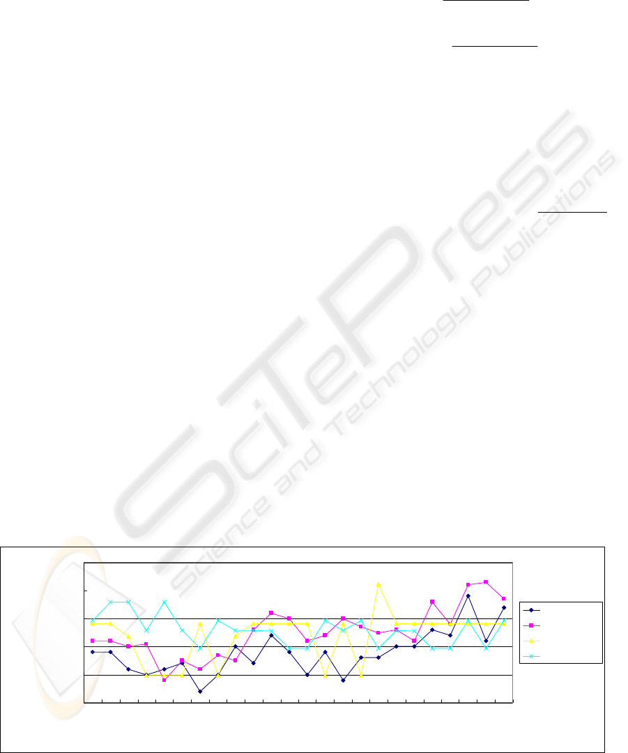
. The predicted
results from different models are all shown in Figure
2. Interestingly, the sum of square errors of affinity
model is 566, which is smaller than those of NN
models (780 and 932). NN1 model is trained for 100
runs, NN2 model is trained for 500 runs. This hints
there could be a unknown pattern within the patient
arrival curve (from 00:00 am to 23:00 pm). Our
affinity model is able to catch such a special pattern
in time series. Of course, the NN model could be
restructured for better competence advantage later.
For example, integrating affinity concept and NN
altogether could perform better than affinity model
or NN model.
0
5
10
15
20
25
1 2 3 4 5 6 7 8 9 101112131415161718192021222324
Hour
Patient Arrival
Actual Data
Af f i ni ty Model
NN1
NN2
Figure 2: Performance Comparison of Different Models.
ICEIS 2008 - International Conference on Enterprise Information Systems
276

4 CONCLUSIONS AND
RECOMMENDATIONS
We proposed a simple prediction method in this
study, although the idea is really simple, it
interestingly performs good. However, pattern could
exist in a very dynamic and complicated form. In
this study, we may be just lucky to find this simple
pattern. A decision maker is encouraged to develop
his/her own perception of closeness/distance in (4)-
(5); thus, various affinity models of data mining are
waiting for exploration.
ACKNOWLEDGEMENTS
This project is under the financial support of
National Science Council, Taiwan (96-2416-H-212-
002-MY2).
REFERENCES
Abdel-Aal, R. E., & Al-Garni, A. Z., 1997. Forecasting
monthly electric energy consumption in eastern Saudi
Arabia using univariate time series analysis. Energy,
Vol. 22, pp. 1059–1069.
Agrawal R. and Srikant.R., 1995. Mining sequential
patterns. In P. S. Yu and A. S. P. Chen, editors,
Proceedings of the 11th International Conference on
Data Engineering (ICDE'95), pp. 3-14, IEEE Press.
TeleTracking, http://www.teletracking.com/ , visited in
2006.
Kim, K. J., & Han, I., 2000. Genetic algorithms approach
to feature discretization in artificial neural networks
for the prediction of stock price index. Expert Systems
with Application, Vol. 19, pp. 125–132.
Kimoto, T., and Asakawa, K., 1990. Stock market
prediction system with modular neural network.
Proceeding of IEEE International Joint Conference on
Neural Network , pp. 1–6.
Larbani, M. and Chen, Y. (2006). Affinity set and its
applications. In Proceeding of the International
Workshop on Multiple Criteria Decision Making, Apr.
14-18, 2007, Poland. Publisher of The Karol
Adamiecki University of Economics in Katowice.
Yu, P. L., 1985. Multiple Criteria Decision Making:
Concepts, Techniques and Extensions. Plenum, New
York.
PREDICTING THE ARRIVAL OF EMERGENT PATIENT BY AFFINITY SET
277