MULTIVARIATE TECHNIQUE FOR CLASSIFICATION RULE

SEARCHING

Exemplieied by CT Data of Patient

Jyhjeng Deng

Industrial Engineering & Technology Management Department, DaYeh University

112 Shan-Jeau Rd., Da-Tsuen, Chang-Hua, Taiwan

Keywords: Correspondence Analysis, Fisher’s linear Discriminant function, multivariate categorical data, parallel

coordinate plots.

Abstract: In the process of searching classification rules for multivariate categorical data, it is crucial to find a quick

start to locate the combination of levels of input and response variables which can contribute to the most

correct classification rate for the response variable. Fisher’s linear discriminant function is proposed to

select some important input-variable candidates; then, correspondence analysis is used to ascertain that the

level of candidates is closely related to the appropriate level of response variable. The closest linkage

between input variable and response variables is chosen as the rule for each input-variable candidate. The

algorithm is applied to the hospital data of patients whose CT scan diagnosis awaits a decision. The result

shows that my algorithm is not only quicker than an exhaustive search but the result is also identical to the

optimum solution by exhaustive search in terms of the correct classification rate. The correct classification

rate is about 80%. Finally, two parallel coordinate plots of the 20% mistakenly classified data and the

corresponding correctly classified data are compared, showing their mutual confounding and explaining

why the correct classification rate cannot be further improved.

1 INTRODUCTION

Patients sent to the emergency unit of a hospital

need immediate care to save their life. To attend to

patients in an appropriate manner, correct treatment

is crucial, leading to the issue of making a correct

diagnosis. In this investigation a data set on 959

patients sent to a local hospital within a certain

period of time for emergency care is collected. The

on duty physicians face the decision whether the

patients need head-computed tomography (HCT),

more commonly known as computed axial

tomography (CAT or CT scan). Since each patient

differs, a rule based on the physical characteristics

(such as blood pressure, breath, mental status, and

triage level, etc.) of the patient should be formulated

to help the physician make an appropriate decision

on the need for HCT. The first 80% (767) of the

original data is used as a training set to establish the

rule; whereas, the second 20% (192) is used as test

data to demonstrate the effectiveness of the rule.

The data set contains seven independent

variables, A1-A7 (such as sex, age, triage level,

mental status, breathing rate, diastolic blood

pressure and pulse rate) and one response variable,

HCT (D). The medical data are further classified by

the physician as in the contingency table shown in

Table 1 in Appendix A. Note that D has two

meanings: (1) the response variable of the HCT,

being the highest standard determined by the on-

duty physician, and (2) the result determined by the

classification rule. At first the double meaning might

be somewhat confusing, but it eliminates the need to

define another variable, as should be clear from the

context as this report proceeds.

A simple and direct way to solve the problem is

enumeration, an exhaustive method. In the single-

variable rule search, there will be

ways to

classifiy a categorical input variable with p levels

into a response variable of 2 levels . For example, to

find the best rule for variable A3 (with three levels)

which will provide the most correct classification via

HCT (with two levels), the correct rate for the

following six rules must be computed: (A3=1, D=1),

(A3=1, D=2), (A3=2, D=1), (A3=2, D=2), (A3=3,

D=1), (A3=3, D=2). Since there are seven

278

Deng J. (2008).

MULTIVARIATE TECHNIQUE FOR CLASSIFICATION RULE SEARCHING - Exemplieied by CT Data of Patient.

In Proceedings of the Tenth International Conference on Enterprise Information Systems, pages 278-286

DOI: 10.5220/0001723702780286

 SciTePress

independent variables and each is classified as 2, 5,

3, 4, 3, 3 and 4 levels, 2*(2+5+3+4+3+3+4)=48

rules need to be evaulated. The classification rule

(A3=1, D=1) means that if the patient’s triage level

is 1, he/she needs to have the HCT. This decision is

applied to the training data; however, it may be

incorrect according to the criterion of response

variable D. Thus, a correct rate can be calculated,

and the highest correct rate chosen. In this case,

when dealing with only one independent variable,

the obtained rule is applied to the test data set to

determine whether this rule can render a similar

correct classification rate. This type of selection

procedure can be applied to the two independent

variables. When variable

x has

l levels and

variable

x has

l levels, then there are 2

rules to be evaluated. In this case study, there will be

2*(2*5+2*3+2*4+2*3+2*3+2*4+5*3+5*4

+5*3+5*3+5*4+4*3+4*3+4*4+3*3+3*4+3*4)= 404

rules altogether. Clearly, evaluating each in

succession is very time consuming; therefore, a

faster, more reliable method should be sought. For

this purpose, two multivariate techniques are used to

solve the problem in sequence. First, Fisher’s linear

discriminant function is built and important input

variables selected. By following the correspondence

analysis, the level from the input variable closest to

the level of the response variable can be selected as

the classification rule. For example, variable triage

(A3) is considered to be one of the most important

of the seven independent variables. Then, a

Euclidean distance can be derived between the level

of independent variable A3 and the level of decision

variable D. The shortest distance between them is

chosen as the classification rule for input variable

A3. By extending the aforementioned procedure for

a single variable to two variables, a combination of

composite rules to determine the optimum correct

classification rate can be established, in this case

about 80%. Finally, two parallel coordinate plots of

the 20% mistakenly classified data and the

corresponding correctly classified data are compared,

showing their mutual confounding and explaining

why the correct classification rate cannot be further

improved. Although Fisher’s linear discriminant

function and correspondence analysis are two well

known techniques in multivariate analysis, using

them together to find the classification rule for

multivariate categorical data is unusual. Fisher’s

function is mostly used to classify multivariate

continuous data into various categories. In the

literature, one can find its application to face

detection (

Yang, Kriegman and Ahuja, 2001) and its

combination with linear programming (

Lam and Moy,

2003). Used to detect the root of two categorical

variables. Correspondence analysis can be used in

the ecological study of animal populations (

Allombert,

Gaston and Martin, 2005

2 FISHER’S LINEAR

DISCRIMINAT FUNCTION

Suppose that there is a sample data set X of

multivariate variable

x composed of samples

with sample size of

n , 1, 2, ,j J= L , from

populations. To obtain the optimum classification

rule for multivariate sample

X , Fisher suggests

finding the linear combination of

ax which

maximizes the ratio of between-group-sum of

squares to the within-group-sum of squares (Hardle

and Simar, 2003),

aBa

aWa

, (1)

where

B is the between-group-sum of squares,

defined as (Johnson and Wichern, 2003)

()()

ii i

B nx x x x

=−−

∑

; (2)

whereas,

W is the within-group-sum of squares,

defined as

()()

ijiiji

Wxxxx

=−−

∑∑

. (3)

Note that

x represents the

j sample from

population

i ;

x , the sample mean of population i ;

, the grand average of the total samples. The

solution of vector

a is found in Theorem 1 (Hardle

and Simar, 2003).

Theorem 1. The vector

a that maximizes (1) is the

eigenvector of

−

corresponding to the largest

eigenvalue.

Now, the pertinent discrimination rule is as follows:

Classify

x into group j where

ax is closest to

ax. When J =2 is grouped, the discriminant rule

is computed as follows: The corresponding

eigenvector in Theorem 1 is

()aW x x

−

=−.

The corresponding discriminant rule is

279

MULTIVARIATE TECHNIQUE FOR CLASSIFICATION RULE SEARCHING - Exemplieied by CT Data of Patient

()

if 0

xaxx

→Π − >

→Π − ≤

, (4)

where

Π represents population i .

Note that all the data are not assumed to be normal;

the only assumption is that they are real numbers.

After this short introduction to Fisher’s linear

discriminant function, the focus is now directed

toward its application to the hospital data. To sketch

the eight variables of 767 data set, parallel

coordinate plots are used. The result is shown in

Appendix B. Since variable A1 is nominal and the

analysis in Appendix B indicates that variable A1

has no strong correlation with variable D. Fisher’s

linear discriminant function with input variables

(A2-A7) is found. Vector

a is [0.00023445, -

0.00079367, 0.00062467, 0.0020182, -2.9766e-06, -

0.00035162]

; the grand average

is [3.4433,

1.7901, 1.1917, 1.9974, 2.9126, 2.3051], the values

a and

corresponding to variables A2-A7.

Then, the number of individuals coming from

which have been classified into

Π by

n , are

denoted. By applying the discriminant rule in Eq. (1)

to the test data set, one has

n =0 and

n =48, the

correct classification rate being 0.75. By examining

the magnitude of the coefficients in

a , it is clear

that the three most important variables are A5

(breathing), A3 (triage) and A4 (mental state);

whereas, the least important is A6 (blood pressure).

Thus, the correlation between the level of these

variables and the CT level is investigated and the

closest relationship between them in terms of the

Euclidean distance searched. The closest is chosen

as the rule to classify the patients who need HCT. A

detailed explanation follows.

3 CORRESPONDENCE

ANALYSIS

The aim of correspondence analysis is to develop

simple indices showing relationships between the

rows and columns of a contingency table, wherein

row and column represents one category of the

corresponding variables. The entry

in table

(with dimension (nxp)) represents the number of

observations in a sample which simultaneously fall

in the i

row category and the j

column category,

for

1, 2, ,in= L and 1, 2, ,

L . Then the

association between the row and column categories

can be measured by an

-test statistic defined as

()

/ ,

ij ij ij

=−

∑∑

(5)

where

= with

represents the sum in

the i

row;

, the sum in the j

column; and

.. .

∑

, the grand total. Under the hypothesis of

independence,

has an

(1)( 1)np

−−

distribution. If

the test statistic

is significant at the 5% level,

investigating the special reasons for the departure

from independence is worthwhile. To extract the

elements of dependence, the principle of

correspondence analysis (CorrAna) is brought into

play. The CorrAna procedure first determines the

SVD (singular value decomposition) of matrix

(nxp) with elements (Hardle and Simar, 2003)

(

)

1/2

ij ij ij ij

cxEE=− . (6)

When assuming that the rank of

C is

, the SVD

C yields

ΓΛΔ , (7)

where

contains the eigenvectors

(nx1) of

CC ,

the eigenvectors

(px1) of

where

1,2,…,R and

()

1/2 1/ 2

diag , ,

λλ

Λ= L

(where diag represents the diagonal matrix) with

12 R

λλ

≥≥≥L (the eigenvalues of

CC ). By

defining the matrices

A (nxn) and

(pxp) as

(

)

()

diag and diag

xB x==, (8)

one can calculate

r (nx1) and

s (px1),

1, 2, ,kR

L as

1/ 2

kk k

−

(9)

where point vectors [

r ,

r ] and [

s ,

s ] are

plotted onto a two-dimensional graph, called biplot,

with n points in point vector [

r ,

r ] representing

the n rows and p points in [

s ,

s ] representing the

p columns. Thus, the entire contingency table can be

simplified as n+p points on the 2D graph. The

ICEIS 2008 - International Conference on Enterprise Information Systems

280

relationship between n points [

r ,

r ] and p points

[

s ,

s ] explains why rows and columns are not

independent.

Now, the correspondence analysis (CorrAna) is

applied to the contingency table of variables A5 and

D as an illustration, shown in Table 1.

Table 1: Contingency table of variables A5 and D for 767

Data.

HCT (D)

1 2

Breath

(A5)

<10/min 1 4

10~24/min 249 510

>24/min 3 0

The corresponding

R of

for Table 1 is 1;

moreover, vector

r =[-0.2762, -0.0038143, 1.4253]

and vector

s =[0.13109, -0.064523]. Since R =1,

there are no

r and

s . A zero vector is substituted

for

r and

s to make a 2D biplot, shown in Fig. 1.

Figure 1: Biplot of variables A5 and D.

Note that the two levels of response variable D

(CTYes corresponding to HCT [D=1] and CTNo,

HCT [D=2]), are close to the second level of

independent variable A5. Examining the value of

(representing A5) and

s (representing D), one may

clearly observe that HCT (D=2) is closer to (A5=2)

than HCT (D=1). The value of HCT (D=2) in Figure

1 is -0.064523, being the second value in

s ; the

value of (A5=2), -0.0038143, being the second value

r ; the value of HCT (D=1), 0.13109, being the

first value in

s . The rule is then derived as if

(A5=2); therefore, HCT should not be administered.

Thus when the breathing level is normal, the patient

does not need HCT. By applying this rule to the

remaining test data, one has

n =0 and

n =47, the

correct rate being 0.75521. Table 1 clearly indicates

that the rule is optimum; hence, any other rule will

yield a worse correct rate. The effectiveness of

applying this rule to the test data can be clearly

observed by scrutinizing the contingency table of

variables A5 and D for the test data set, shown in

Table 2.

Table 2: Contingency table of variables A5 and D for 192

Data.

HCT (D)

1 2

Breath

(A5)

<10/min 1 0

10~24/min 47 144

>24/min 0 0

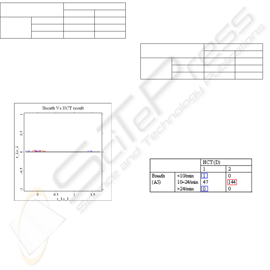
The rule can be applied to Table 2 to obtain Figure 2,

where the correct result from the main rule （if

[A5=2] then do not administer HCT） is marked in

red; whereas, the correct result from the congruent

rule （if [A5≠ 2] then administer HCT） is marked

in blue. The correct rate is (1+0+144)/192=0.75521.

No other classification rule will result in a better

correct rate.

Figure 2: Classification rule with contingency table.

By applying the same procedure to the contingency

tables of variables A3 and D, and A4 and D, the

correct rates of 0.70312 and 0.72396, respectively,

are obtained. The rules derived are if (A3=1), then

HCT (D=1); and if (A4=2), then HCT (D=1),

respectively. These values indicate that when the

triage level is 1, the patient needs HCT; and when

the mental status is ‘to call’, HCT, respectively. The

corresponding biplots are shown in Figures 3 and 4.

For the sake of analytical completeness, the

contingency tables of variables A1-A7 vs D for both

the training and the test data sets are listed in

Appendix C.

281

MULTIVARIATE TECHNIQUE FOR CLASSIFICATION RULE SEARCHING - Exemplieied by CT Data of Patient

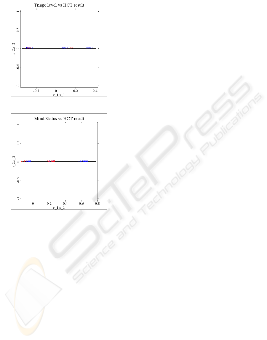
Figure 3: Biplot of variables A3 and D.

Figure 4: Biplot of variables A4 and D.

From the data reported in Appendix C and previous

results, one may assert that analysis by Fisher’s

linear discriminant function and CorrAna provides a

quick start for identifying the important input

variables for searching the classification rule. In this

case the important input variables are A3, A4 and

A5, being in agreement with the Chi-squares test on

the contingency table shown in Appendix C.

Furthermore, the rule provided by CorrAna is in

very strong agreement with the exhaustive search,

with only a small difference in the rule for A4. The

rules by CorrAna for each important variable are: if

A3=1 then D=1; if A4=2, then D=1; if A5=2 then

D=2. These rules differ from the ones obtained by

exhaustive search only in variable A4, where if

A4=1 then D=2; however, there is no difference in

the correct classification rate.

The optimum correct classification rate by the

single-variable classification rule is 0.75521,

provided by the rule of input variable A5, where if

(A5=2) then D=2. Further research is needed to find

composite classification rules for two variables

which, perhaps, would render a higher correct rate.

The result of two-variable classification is explained

below and listed in the combination of composite

rules.

4 OPTIMUM RULE OF

COMBINATION FOR TWO

VARIABLES

Following the previous arguments, the combination

rule for two variables is straightforward. For the

sake of simplicity, only the procedure for finding the

optimum correct rate is illustrated. Variables A3 and

A4 are used to form a new variable, A9, where

A9=(A3-1)*4+A4. (10)

Here A9, A3 and A4, in addition to designating

the composite variable name, triage and mental

status, also represent the level of the corresponding

variables. Since the level of variable A3 is three and

that of A4 is 4, the level of A9 indicates the

combination level of A3 and A4, as shown in

equation (10). For example, when A9=9 the equation

denotes that A3=3 and A4=1. Theoretically, the total

level of A9 is 12; however, in this case study it is

only 10 because levels 11 and 12 of A9 are missing.

Therefore, the frequencies of (A3=3 and A4=3) and

(A3=3 and A4=4) are zero with regard to both levels

of HCT response variable (D). Applying CorrAna to

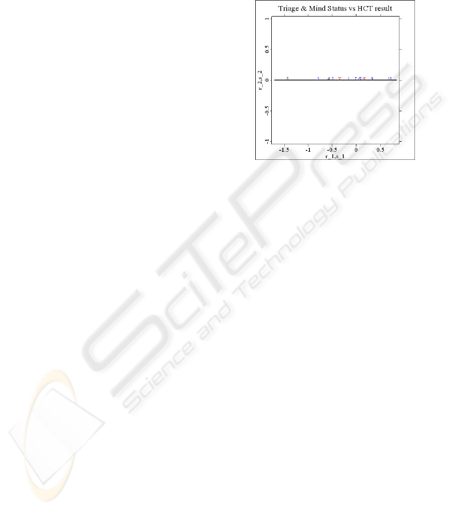
A9 with regard to response D, the biplot shown in

Figure 5 is obtained.

For a clearer display, the labels of the levels of

response D are changed from ‘CTYes’ and ‘CTNo’

to ‘Y’ and ‘N’. It is clear from Figure 5 that levels 8,

3, 4 and 2 are located to the left of ‘Y’ and levels 10

and 9 to the right of ‘N’; whereas, the other levels

remain between ‘Y’ and ‘N.’ Thus, it can be said

that when (A3=2 and A4=4) or (A3=1 and A4=3 or

4 or 2), then one should judge D=1; whereas, when

(A3=3 and A4=2) or (A3=3 and A4=1), then D=2.

Therefore, when the triage level is 2 and the mental

status level is a coma, or when the triage level is 1

and the mental status is unclear, one should judge

HCT to be necessary. In such cases, the patients are

in serious conditions; thus, administering HCT is

appropriate and useful in diagnosing the root

problem. However, when patient is in a level 3 triage

and the mental status is clear or one capable of

responding to a verbal stimulus, HCT is unnecessary.

Note that in these two cases, the patients are in better

condition, but that many patients do not fall into

either of these stated categories. To overcome this

ICEIS 2008 - International Conference on Enterprise Information Systems

282

problem, the single rule of （ if A5=2, D=2 ）is

applied to the remainder.

It is worth noting that the single variable rule, the

shortest Euclidean distance between the levels of the

independent and the response variables is chosen as

the classification rule; whereas, in the two-variable

rule, the levels of the composite formed by the two

variables on each side of the response variable is

chosen as the composite rule. These principles are

true because in the single-variable case, once the

main classification rule has been set, its complement

(congruent) is automatically determined. For

example, in the case of A5 and D, as shown in

Figure 2, once the main rule, if (A5=2) then D=2, is

set, its complement, if (A5 ≠ 2) then D=1, is

automatically determined. Note that (A5≠ 2) means

that (A5=1 or 3). Therefore, once the destiny of

(A5=2) is determined as D=2, the other choices of

A5 have a pre-determined result. Thus, a reasonable

choice for the classification rule can be based on the

shortest linkage between the levels from the

independent and the response variables.

If the same argument is followed in the two-

variable case, then there is only one level in the

composite variable A9 which can be associated with

one of the two levels of D. The other values of A9

will be assigned with the alternative value of D, a

procedure which does not make good sense since the

other values are not necessarily exclusive with the

chosen value in the main rule. To clarify this point,

an illustrative example is given as follows. If the

shortest distance between level 5 of A9 and level 2

of D is chosen as the classification rule, then by the

same argument in single-variable, level 5 of A9

should be associated with level 2 of D and other

values (these include level 9, of course) of A9

should be with level 1 of D. However, Figure 5

clearly shows that level 9 of A9 should be associated

with level 2 of D since it is closely associated with

level 2 of D by the interpretation of correspondence

analysis (Hardle and Simar, 2003). Thus, the only

reasonable classification rule is to divide the levels

of the composite variable into three regions with the

levels of D as the demarcation points. With the

levels in the middle region undecided, the levels in

the left region are associated with the left

demarcation point; whereas, the levels in the right

region are assigned to the right extremity. Note also

that the levels in the middle region can be classified

later by the rule derived from the single variable.

The optimum correct classification rate by these

two-variable classification rules in addition to the

single rule is 0.76562, with

n =2 and

n =43. A

slightly better result is achieved than from the single

variable rule where the correct classification rate is

0.75521, with

n =0 and

n =47.

Figure 5: Biplot of variables A9 and D.

By examining the two misclassifications of

n ,

one finds an additional rule to eliminate

n : When

(A3=1, A4>=3, A6=3) then D=2. This means that

when the triage level is 1, the mental status is ‘to

pain’ or ‘coma’, and the diastolic blood pressure is

above 110 mm Hg (very serious high blood

pressure), the patient should not be administered

HCT because the situation is probably too dangerous.

This is a special provision under the rule of stating

that when (A3=1, A4>=3) then D=1, thereby

indicating the importance of abnormally high

diastolic blood pressure, a strong indicator to

overrule the HCT decision under serious health

conditions.

At this point, the correct classification rate is

0.77604, with

n =0 and

n =43. Note that

means the number of misclassified members,

thereby these members are treated as not

administering HCT (D=2) when in fact they need for

administering HCT (D=1). Misclassifying D=1 as

D=2 is more serious than that of D=2 as D=1 since

the penalty for the former error is life or death;

whereas, the consequence of the latter is merely a

waste of CT resource utilization. Note that of 192

patients only 48 patients were classified as D=1;

moreover, of these 48, the classification was correct

only five times. Since correct classification rate for

the 48 patients was very low, it is worthwhile to

investigate why

n cannot be reduced. By

examining the sorted data of

n =43, one notices

283

MULTIVARIATE TECHNIQUE FOR CLASSIFICATION RULE SEARCHING - Exemplieied by CT Data of Patient

that the age factor has been overlooked. When

considering the age factor (A2), a new rule is

formulated to reduce

n : when (A2=5, A3=1,

A6=3) then D=1. This means that when the patient’s

age is above 65 years, the triage level is 1, and the

diastolic blood pressure is above 110 mm Hg, the

patient should be administered HCT. When this rule

is applied in addition to the previous composite rules,

the correct classification rate is increased to 0.79167,

with

n =1 and

n =39. The result of

n =1 is an

exception to the previous rule. Apparently, nothing

can be done to further reduce the

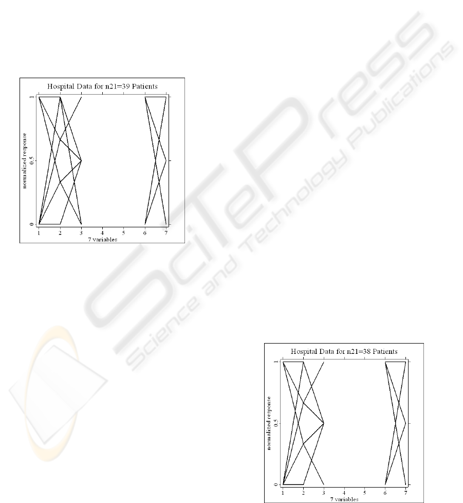
n . The parallel

coordinate plot (PCP) of seven variables (A1-A7)

for the data of

n =39 is shown in Figure 6.

Figure 6: Parallel coordinate plots of 39 hospital data.

Several points are noteworthy. First, in comparison

with Figure B1, Figure 6 has only one colour (black)

since the data of

n =39 are members of D=1 only.

Second, there is no connection between variables A3

through A6, thereby, indicating that the levels of A4

and A5 are of single value. Indeed, A4=1 and A5=2,

thus indicating that patients having a clear mental

status and a normal breathing rate are easily

misclassified as not needing HCT, an understandable

error. Third, there are four age levels (2-5) instead of

the five in the original setting. Each age level is

connected with two triage levels except for age level

2 of which is connected to only triage level 2. In

comparison with the PCP in Figure B1, the pattern

in Figure 6 is quite different, wherein each age level

is connected to almost every triage level. Fourth, the

diastolic blood pressure is shown only for levels 2

and 3, thereby indicating that none of the patients

has normal blood pressure. Moreover, the pulse

levels are at 1-3, thus indicating that none of the

patients has an unusually high pulse rate (greater

than 120/min). Furthermore, there is no connection

between A6=2 and A7=1, thereby indicating that no

patient has blood pressure in the range of 80 to 110

mm Hg and a pulse rate lower than 60/min.

After a close examination of the sorted 39 data

sets, another rule is discovered: if (A2=5, A3=1,

A4=1) then (D=1). This rule indicates that when the

patient is very old (more than 65 years) and has a

triage level of 1 and a clear mental status, HCT

should be administered. This rule will reduce one

mistake in

n , thereby rendering the correct

classification rate of 0.79688 with

n =1 and

n =38, the optimum discoverable solution. The

PCP of the

n =38 data set is shown in Figure 7.

When comparing Figures 6 and 7, one notices that

the line connecting the normalized value of A2=1 to

A3=0 in Figure 6 has been deleted from Figure 7.

There is no observable distinction between D=1

from 38 patients and D=2 from 122 patients,

extracted from 144 data sets, wherein D=2 in the test

data has the response variable D=2 with A2>1 and

A4=1 and A5=2 and A6>1 and A7<4. The

aforementioned conditions set for D=2 are exactly

the same as for the 38 sets except for D=1. The PCP

of the 122 sets is shown in Figure 8. When

comparing Figures 7 and 8, it is clear that if the line

segments in each Figure are treated as elements in a

set, then Figure 7 can be regarded as contained in

Figure 8 in terms of the set concept, thereby

demonstrating that since the 38 sets are prominently

involved with the corresponding 122 sets, the two

cannot be separated by any rule. For the sake of

completeness, part of the XploRe (Hardle, Klinke

and Muller, 2000) code is listed to illustrate the

formulation of the composite rule in Appendix D.

The self-explanatory code is similar to the c code.

Figure 7: Parallel coordinate plots of 38 hospital data.

ICEIS 2008 - International Conference on Enterprise Information Systems

284

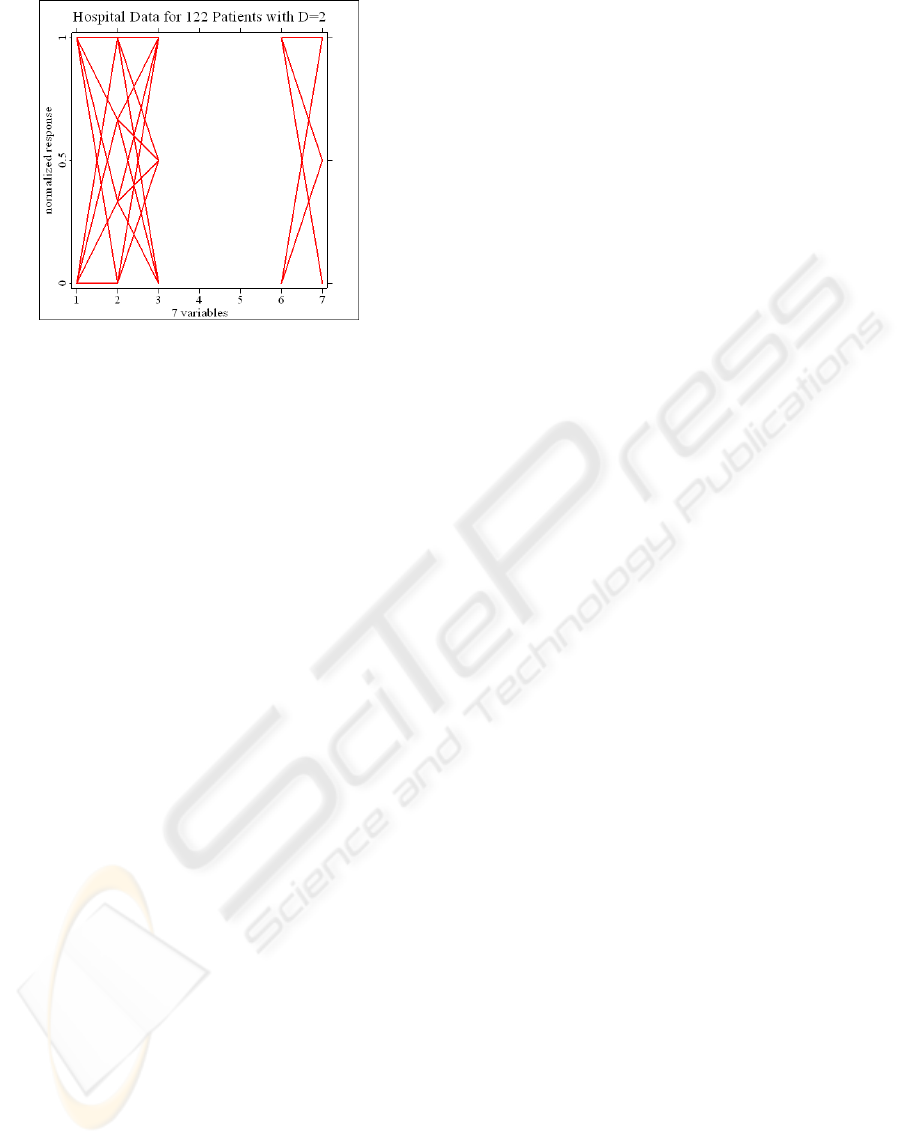
Figure 8: Parallel coordinate plots of 122 hospital data.

5 CONCLUSIONS

Two multivariate techniques have been proposed to

clarify patients sent to an emergency room to wait

for a decision on the administration of HCT. The

959 data set were segmented into two portions, a

767 training data set and a 192 test data set, after

which Fisher’s linear discriminant function was used

to find linear rule vector

a . Since classification

using rule vector

a in equation (4) is not practical

for on-duty physicians, three important variables,

such as triage (A3), mental status (A4) and breathing

rate (A5), were chosen on the basis of the magnitude

of the coefficients of

a . Next, correspondence

analysis was used to determine the simple

classification rule most suitable for each variable to

classify the need for administering HCT. The simple

classification rule has the format of （if A5=x then

D=y）where x and y are the levels of the input (A5)

and output (D) variables, respectively. The selection

of the rule is based on the shortest Euclidean

distance between the levels of the input variable

(e.g., A5) and response variable D located on the x-

axis of a biplot. The case study demonstrated that

output from the joint effort of the multivariate

technique coincided with the exhaustive search, a

promising result. The optimum correct rate is only

0.75521 with

n =0 and

n =47 for the rule of (if

A5=2 the D=2), meaning that if the patient’s

breathing rate lies within the normal range of

10~24/min, HCT is not needed.

The extension of a single-variable classification

rule to a two-variable one is straightforward, yet

requiring a small modification for choosing the rule.

First, a composite variable (e.g., A9) is formed by a

linear combination of the two variables based on

equation (10) so that each combination of the levels

from the two maps into an integer level of the

composite variable. Then typical CorrAna is applied

to the contingency table formed by variables A9 and

D, wherein a biplot is produced with points

representing both the levels of the composite

variable and response variable D. By taking the two

points of the levels of D as the demarcation points,

the x-axis can be cut into three regions: one to the

left of the left extremity, the second between the

demarcations, and the third to the right of the right

extremity. Moreover, the levels in the left regions

are assigned to the level of D at the left demarcation

point, the levels in the right regions to the level of D

at the right demarcation point, and the levels of the

composite variable between to the level of D on the

basis of the optimum classification rule from the

single variable. The two variables selected are triage

(A3) and mental status (A4), which render the

highest correct classification rate among all

combinations of two variables. The rules state that

when (A3=2 and A4=4) or (A3=1 and A4=3 or 4 or

2) D=1; whereas, when (A3=3 and A4=2) or (A3=3

and A4=1), D=2. Thus, the correct classification rate

is 0.76562 with

n =2 and

n =43.

The correct classification rate can be further

increased by examining the structure of the sorted

but misclassified items in the test data set. The

formulation of the composite rule for the case study

is listed in Appendix D, with the correct

classification rate of 0.79688 with

n =1 and

n =38. The composite rules may be generally

summarized as (1) when the triage level is 2 and the

mental status is a coma, or when the triage level is 1

and the mental status is unclear, HCT should be

administered, and (2) when the patient is in level 3

of triage and the mental status is one capable of

responding to a verbal stimulus, HCT is unnecessary.

Exceptional rules should be applied to patients older

than 65 years (A2) and those with high diastolic

blood pressure (A6). For example, (1) when the

triage level is 1, the mental status is ‘to pain’ or

‘coma’, and the diastolic blood pressure is above

110 mm Hg (seriously high), the patient should not

be administered HCT; (2) when the patient’s age is

older than 65 years, the triage level is 1, and the

diastolic blood pressure is above 110 mm Hg, the

patient must be administered HCT. It is noteworthy

that the variables of sex (A1) and pulse rate (A7) are

not considered in the composite rules.

285

MULTIVARIATE TECHNIQUE FOR CLASSIFICATION RULE SEARCHING - Exemplieied by CT Data of Patient

To show why the correct classification rate cannot

be increased, two parallel coordinate plots of

the

n =38 data set being in D=1 and the

corresponding 122 data set being in D=2 were

compared. The two data sets had the same domains

for variables A1-A7. The comparison indicated that

since both are prominently involved (highly similar),

they cannot be separated by any rule. Thus, no

improvement can be made in the correct

classification rate.

ACKNOWLEDGEMENTS

I grateful thank my colleague Prof. Paul Chen for

both encouraging me to pursue this research and

generally sharing his hospital data. I also express

appreciation to Dr. Cheryl Rutlede, Department of

English, DaYeh University, for her editorial

assistance.

REFERENCES

Yang, M., Kriegman, D and Ahuja, N., 2001, Face

Detection Using Multimodal Density Models,

Computer Vision and Image Understanding 84, 264–

284.

Lam, K. and Moy, J., 2003, A piecewise linear

programming approach to the two-group discriminant

problem

–

an adaptation to Fisher’s linear

discriminant function model, European Journal of

Operational Research 145, 471– 481.

Allombert, S., Gaston, A. and Martin, J., 2005, A natural

experiment on the impact of overabundant deer on

songbird populations, Biological Conservation 126,

1– 13.

Hardle, W. and Simar L., 2003. Applied Multivariate

Statistical Analysis, Springer. Berlin.

Johnson R. and Wichern D., 2002, Applied Multivariate

Statistical Analysis, Prentice Hall. 5

, NJ, USA.

Hardle, W., Klinke, S. and Muller M., 2000. XploRe

Learning Guide, Springer. Berlin.

ICEIS 2008 - International Conference on Enterprise Information Systems

286