
Neural Approaches to Image Compression/
Decompression Using PCA based Learning Algorithms
Luminita State
1
, Catalina Cocianu
2
, Panayiotis Vlamos
3
and Doru Constantin
1
1
Department of Computer Science, University of Pitesti, Pitesti, Romania
2
Department of Computer Science, Academy of Economic Studies, Bucharest, Romania
3
Department of Computer Science, Ionian University, Corfu, Greece
Abstract. Principal Component Analysis is a well-known statistical method for
feature extraction, data compression and multivariate data projection. Aiming to
obtain a guideline for choosing a proper method for a specific application we
developed a series of simulations on some the most currently used PCA
algorithms as GHA, Sanger variant of GHA and APEX. The paper reports the
conclusions experimentally derived on the convergence rates and their
corresponding efficiency for specific image processing tasks.
1 Introduction
Principal component analysis allows the identification of a linear transform such that
the axes of the resulted coordinate system correspond to the largest variability of the
signal. The signal features corresponding to the new coordinate system are
uncorrelated. One of the most frequently used method in the study of convergence
properties corresponding to different stochastic learning PCA algorithms basically
proceeds by reducing the problem to the analysis of asymptotic stability of the
trajectories of a dynamic system whose evolution is described in terms of an ODE [5].
The Generalized Hebbian Algorithm (GHA) extends the Oja’s learning rule for
learning the first principal components. Aiming to obtain a guideline for choosing a
proper method for a specific application we developed a series of simulations on some
the most currently used PCA algorithms as GHA, Sanger variant of GHA and APEX.
2 Hebbian Learning in Feed-forward Architectures
The input signal is modeled as a wide-sense-stationary n-dimensional process
()()
0≥t,tX of mean 0 and covariance matrix
(
)
(
)
(
)
StXtXE
T
= . We denote by
n
,...,ΦΦ
1
a set of unit eigen-vectors of S indexed according to the decreasing order
of their corresponding eigen-values
n
λ
≥≥
λ
≥
λ
L
21
. The most informative
State L., Cocianu C., Vlamos P. and Constantin D. (2008).
Neural Approaches to Image Compression/Decompression Using PCA based Learning Algorithms.
In Proceedings of the 8th International Workshop on Pattern Recognition in Information Systems, pages 187-192
Copyright
c
SciTePress

directions of the process
(
)()
0≥t,tX are given by
n
,...,
Φ
Φ
1
and for any
nmm ≤≤1, its LMS-optimal linear features are
m
,...,
Φ
Φ
1
. The architecture of a
PCA neural network consists of the n-neuron input layer and the m-neuron
computation layer. The aim is to develop an adaptive learning algorithm to encode
asymptotically
m
,...,ΦΦ
1
as values of the synaptic vectors
m
W,...,W
1
of the neurons
in the computation layer. Let
(
)
(
)
(
)
(
)
tW,...,tWtW
m1
=
be the synaptic memory at the
moment t, and let
()
(
)
(
)
(
)
T
m
tY,...,tYtY
1
= be the output of the computation
layer, mj ≤≤1 ,
() () ()
tXt
T
j
Wt
j
Y = . The Hebbian rule for learning the first principal
component is,
() ()
(
)
(
)
(
)
kYkXkkWkW
111
1
η
+
=+ , where the sequence of learning rates
()()
kη are taken such that the conditions of the Kushner theorem hold [5],
()
∞=η
∑
∞
=1k
k ,
()
0=
η
∞→
klim
k
, there exists 1p > such that
()()
∞<η
∑
∞
=1k
p
k . The
normalized version of the Hebbian learning rule is,
()
(
)
(
)
(
)
(
)
() () () ()
kYkXkkW
kYkXkkW
kW
11
11
1
1
η
η
+
+
=+
(1)
In order to get a local learning scheme a linearized version of (1) using first order
approximation was proposed in [7] yielding to the cellebrated Oja’s learning
algorithm,
() ()
(
)
(
)
(
)
(
)
(
)
(
)
kWkYkYkXkkWkW
1
2
1111
1 −+=+
η
(2)
The Generalized Hebbian Algorithm (GHA)
[3] is one of the first neural models
for extracting multiple PCs. At any moment t, each neuron j,
1≥j , receives two
inputs, the original signal X(t) and the deflated signal X
j
(t) and computes
() () ()
tXtWtY
T
jj
= and
()
(
)
(
)
tXtWtY
j
T
jj
~
~
= ,
(
)
(
)
(
)()
tWtYtXtX
jjjj 111
~
~
−−−
−= , 2≥j .
The GHA learning scheme is, for
mj
≤
≤
2 ,
() ()
(
)
(
)
(
)
(
)
(
)
(
)
kWkYkYkXkkWkW
1
2
1111
1 −+=+
η
(3)
() ()
(
)
(
)
(
)
(
)
(
)
(
)
kWkYkYkXkkWkW
jjjjjj
2
~
~
~
1 −+=+
η
(4)
where
() () ()
,kXkWkY
T
jj
=
(
)
(
)
(
)
(
)
=−=
−−−
kWkYkX
~
kX
~
jjjj 111
() ()
∑
−
=
1
1
j
i
ii
kWkY
, and
() () ()
kX
~
kWkY
~
j
T
jj
= .
The variant proposed by Sanger [7] simplifies the learning process by using only
output of each neuron in both, the synaptic learning scheme and the input deflation.
The Sanger variant of GHA is, for
mj
≤
≤
2
,
() ()
(
)
(
)
(
)
(
)
(
)
(
)
kWkYkYkXkkWkW
1
2
1111
1 −η+=+
(5)
() ()
(
)
(
)
(
)
(
)
(
)
(
)
kWkYkYkXkkWkW
jjjjjj
2
~
1 −+=+
η
(6)
188

where
() () ()
kXkWkY
T
jj
= and
(
)
(
)
(
)
(
)
kWkYkX
~
kX
~
jjjj 111 −−−
−= is the input deflated
at the level of the jth neuron.
The APEX learning algorithm proposed in [2] generalizes the idea of lateral
influences by imposing a certain learning process to the weights of lateral connections.
The output of each neuron j, is computed from its own output and the effects of the
outputs corresponding to all neurons i,
11
−
≤
≤
ji , weighted by the coefficients
()
ta
ij
,
() () () () ()
∑
−
=
−=
1
1
j
i
iij
T
jj
tYtatXtWtY
2≥j
(7)
The learning scheme for the local memories is essentially the Oja’s learning rule
taken for the transformed outputs
j
Y ,
()
(
)
(
)
(
)
(
)
(
)
(
)
[
]
tWtYtXtYttWtW
jjjjj
2
1 −η+=+
(8)
The learning scheme for the weights of lateral connections is given by,
()
(
)
(
)
(
)
(
)
(
)
(
)
[
]
tatYtYtYttata
ijjjiijij
2
1 −η+=+
(9)
Note that the theoretical analysis [1], [2], [3], establishes the almost sure
convergence to the principal components of the sequences of weight vectors
generated by the above mentioned algorithms.
3 Recursive Least Square Learning Algorithm of the Principal
Directions
Let W
1
(t-1) be the synaptic vector at the moment t and assume that the inputs are
applied at the moments
t=0,1,2,…. If we denote by X(k) the input at the moment k,
then the output is
Y(k) = W
1
(k-1)h
1
(k) = W
1
(k-1)W
T
1
(k-1) X(k), where h
1
(k)=W
T
1
(k-1)
X
(k) is the neural activation induced by the input. The mean error at the moment t is
() ( )
∑
=
ε=
t
k
ktJ
1
2
1
, where
()
(
)
(
)
2
2
kYkXk −=ε
. The aim is to determine
()
tW
1
ˆ
minimizing
()()
tWJ
11
the overall error, when at each moment of time k, 1
≤
k
≤
t, the
decompression is assumed as being performed using the filter
W
1
(t), that is,
()
(
)
=tWJ
11
() () ()()()()()()
khtWkXkhtWkX
t
t
k
T
11
1
11
1
−−
∑
=
(10)
()
()
()()
⎟
⎠
⎞
⎜
⎝
⎛
=
∈
tWJtW
n
RtW
111
1
infarg
ˆ
,
()
(
)
(
)
() ()
2
11
1
1
ˆ
thth
thtX
tW
T
TT
=
(11)
Denoting by
() ( )
1
1
2
11
−
=
⎟
⎠
⎞
⎜
⎝
⎛
=
∑
t
k
khtP
and
(
)
(
)
(
)
tPthtk
111
=
, we get the RLS algorithm ,
(
)
0
1
W randomly selected; h
1
(t) = W
T
1
(t-1)X(t);
()
(
)()
() ( )
11
1
1
2
1
11
1
−+
−
=
tPth
thtP
tk
189

P
1
(t)=[1-k
1
(t)h
1
(t)]P
1
(t-1);
(
)
(
)
(
)
(
)
(
)( )
[
]
1
1
ˆ
11
1
1
ˆ
1
ˆ
−−+−= tWthtXtktWtW
In case that the largest eigen value
λ
1
of the covariance matrix
Σ
is of multiplicity
order 1 and let
φ
1
be its corresponding unit eigen vector. The theoretical analysis
concerning the behavior of the sequence
(
)
(
)
Nt
tW
∈
1
ˆ
establishes that, almost surely,
If
()()
00
11
>φ
T
W , then
(
)
11
ˆ
lim
φ=
∞→
tW
t
. If
(
)
(
)
00
11
<φ
T
W , then
(
)
11
ˆ
lim
φ−=
∞→
tW
t
.
Let
∑
=
φα=
n
i
ii
ttX
1
)()( be the expansion of the input signal in terms of the
{}
n
φφ ,...,
1
, an orthogonal basis of
Σ
eigen vectors, where the corresponding eigen
values are taken in the decreasing order. Let
∑
−
=
φα−=
1
1
)()()(
p
i
iip
ttXtd be the deflated
signal at the level p,
np ≤≤2 . The extended RLS algorithm for learning the first m
principal components is given by the following learning equations.
h
p
(t)=W
T
(t-1)X(t);
()
(
)
(
)
() ( )
11
1
2
−+
−
=
tPth
thtP
tk
pp
pp
p
P
p
(t)=[1-k
p
(t)h
p
(t)]P
p
(t-
1) ;
() ( ) ()
(
)
(
)
(
)
[
]
1
ˆ
1
ˆˆ
−−+−= tWthtXtktWtW
ppppp
Theoretical analysis establishes that, if
npp
λ
λ
λ
λ
λ
≥≥>>>>
+
LL
121
, then
for each
1≥p , the sequence
(
)
(
)
Nt
p
tW
∈
ˆ
generated by the extended RLS converges to
either
p
φ
or
p
φ
−
.
4 Experimental Analysis and Concluding Remarks
In the following we present the use of above mentioned learning schemes for image
compression/decompression purposes. Let
(
)
tI
be a wide-sense- stationary N-
dimensional process of mean
(
)
(
)
tIE
resulted by sampling a given image
I
;
() () ()
(
)
tIEtItI −=
. Each sampled matrix
(
)
tI is processed row by row, each row
being split in lists of 15 consecutive components. We denote by
(
)
tX such a sub-list
and we assume that
()
tX
~
()
∑
,N 0
. We denote by 15
=
n the dimension of the input
data,
3=m the number of desired principal components,
{
}
75502010 ,,,t
max
∈
the
number of the variants of the image
I,
()
()
tt
t
ln
1
=
η
the sequence of learning rates
taken to satisfy the constrains considered in the Kushner theorem,
()
RMW
x3150
∈
the
initial synaptic memories whose entries are randomly generated; each column vector
of
0
W is of norm 1. In case of the APEX algorithm, the initial values of the lateral
connection weights are
0
=
≥∀
ij
a,ji
and for all
31
≤
<
≤
ji
,
ij
a are randomly
generated according to the uniform distribution on[0,1) . The reported results are
190
obtained with respect to the following examples,
(
)
(
)
(
)
3,2,1,,...,
151
==∑ idiag
ii
i
σσ
,
()
,1.0
1
=
k
σ
()
,6
2
2
=
σ
()
(
)
(
)
(
)
,5
1
3
,10
2
1
1
2
,15
1
1
====
σσσσ
(
)()
04.0,2
22
3
==
k
σσ
() () ()
,1,4
3
3
3
2
3
1
===
σσσ
()
01.0
3
=
k
σ
, 154
≤
≤
k . The empirical mean variation of
the synaptic vectors on the final iteration and the mean error with respect to the eigen
vectors are given by,
()( )()
∑
=
−=
m
i
maximaxi
tW,tWD
m
V
1
1
1
,
()( )( ) ( )() ( )()
∑
=
−−=−
n
k
iiii
ktWktWtWtWD
1
maxmaxmaxmax
11,
()()
∑
=
Φ=
m
i
imaxi
,tWE
m
Er
1
1
,
()() ( )() ()
∑
=
Φ−=Φ
n
k
imaxiimaxi
kktWD
n
,tWE
1
1
.
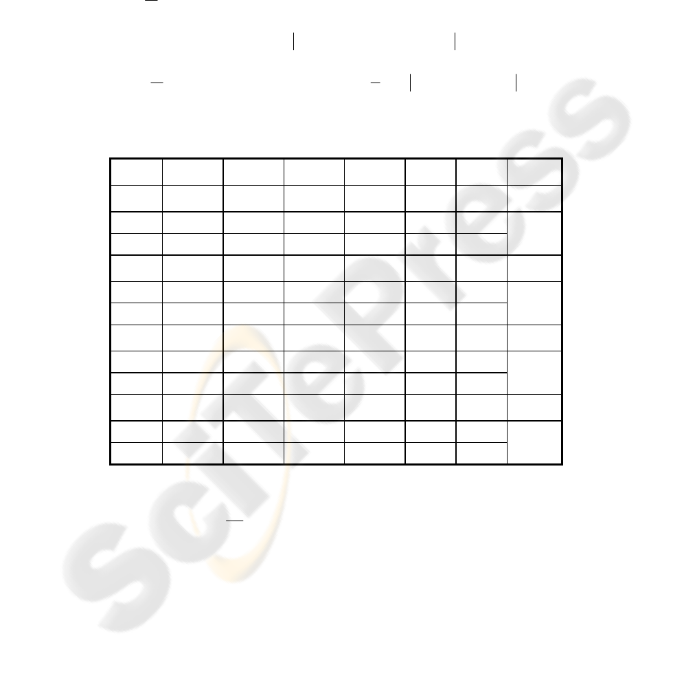
The obtained results are shown in Table 1and Table 2.
Table 1.
V -
GHA
Er-
GHA
V -
Sanger
Er-
Sanger
V-
APEX
Er-
APEX
∑
max
t
0.0377 0.0339 0.0371 0.0423 0.0491 0.0499
1
∑
75
0.0186 0.0295 0.0186 0.0403 0.0243 0.0426
2
∑
0.0064 0.0379 0.0054 0.0532 0.0074 0.0417
3
∑
0.0387 0.0334 0.0393 0.0429 0.0542 0.0485
1
∑
50
0.0276 0.0331 0.0273 0.0450 0.0348 0.0453
2
∑
0.0090 0.0414 0.0070 0.0561 0.0102 0.0442
3
∑
0.0896 0.0417 0.0851 0.0551 0.1085 0.0543
1
∑
20
0.0572 0.0434 0.0499 0.0572 0.0662 0.0505
2
∑
0.0160 0.0484 0.0114 0.0614 0.0172 0.0493
3
∑
0.1569 0.0555 0.1751 0.0612 0.1759 0.0626
1
∑
10
0.0774 0.0629 0.0600 0.0629 0.0858 0.0531
2
∑
0.0202 0.0637 0.0135 0.0637 0.0211 0.0520
3
∑
The entries of
()
RMW
x3150
∈ are randomly generated, but each column of
0
W is
of norm 1. The ratio
E
r
V
of the stabilization coefficient V and the error Er, is fast
decreasing in case of the APEX and GHA algorithms as compared to its variation in
case of Sanger variant. The APEX and GHA lead to smaller errors versus the
stabilization index V. The stabilization of the Sanger variant is installed faster than in
case of GHA and APEX. The errors are significantly influenced by the variation of
the eigen values and they are less influenced by their actual magnitude.
191
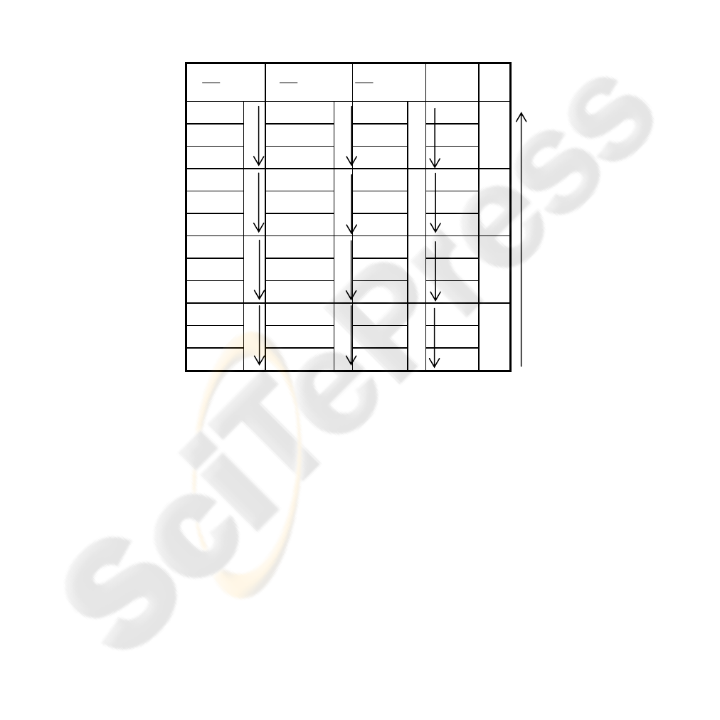
According to the results obtained by our tests we conclude that there are no
significant differences from the point of view of the corresponding convergence rates
between the GHA and the Sanger variant, but the APEX algorithm proves to be
slower than them, most probably because it the convergence rate is more influenced
by the initial values. Also, the performance is strongly dependent on the magnitude
of the noise variances. The tests on the efficiency of the RLS algorithm were
performed on the 10
×10 matrix representations of the Latin letters. The experiments
pointed out that the good quality can be maintained when the
compression/decompression process involved at least the first 15 components. Only 5
line features assure enough accuracy in the compression/decompression process.
Table 2.
E
r
V
- GH
A
E
r
V
-Sange
r
E
r
V
-APE
X
∑
max
t
1.1120 0.8770 0.9839
1
∑
1.1586 0.9160 1.2634
2
∑
2.1486
1.5446 1.9981
3
∑
75
2.8270 2.1320 2.8099
1
∑
0.6305 0.4615 0.6029
2
∑
0.8338
0.6066 0.7682
3
∑
50
1.3179 0.8723 1.3108
1
∑
1.5357 0.9538 1.6158
2
∑
0.1688
0.1015 0.1774
3
∑
20
0.2173 0.1247 0.2307
1
∑
0.3305 0.1856 0.3488
2
∑
0.3899
0.2119 0.4057
3
∑
10
References
1. Chatterjee, C., Roychowdhury, V.P., Chong, E.K.P.: On Relative Convergence Properties
of PCA Algorithms, IEEE Trans. on Neural Networks, vol.9,no.2 (1998)
2. Diamantaras, K.I., Kung, S.Y.: Principal Component Neural Networks: theory and
applications, John Wiley &Sons, (1996)
3. Haykin, S., Neural Networks A Comprehensive Foundation, Prentice Hall,Inc. (1999)
4. Hastie, T., Tibshirani, R., Friedman,J.: The Elements of Statistical Learning Data Mining,
Inference, and Prediction, Springer (2001)
5. Kushner, H.J., Clark, D.S.: Stochastic Approximation Methods for Constrained and
Unconstrained Systems, Springer Verlag (1978)
6. J. Karhunen, E. Oja: New Methods for Stochastic Approximations of Truncated Karhunen-
Loeve Expansions, Proc. 6
th
Intl. Conf. on Pattern Recognition, Springer Verlag (1982)
7. Sanger, T.D.: An Optimality Principle for Unsupervised Learning, Advances in Neural
Information Systems, ed. D.S. Touretzky, Morgan Kaufmann (1989)
192
