
Scoring Systems and Large Margin Perceptron Ranking
using Positive Weights
Bernd-Jürgen Falkowski and Arne-Michael Törsel
University of Applied Sciences Stralsund
Department of Economics
Zur Schwedenschanze 15, D-18435 Stralsund, Germany
Abstract. Large Margin Perceptron learning with positive coefficients is
proposed in the context of so-called scoring systems used for assessing
creditworthiness as stipulated in the Basel II central banks capital accord of the
G10-states. Thus a potential consistency problem can be avoided. The
approximate solution of a related ranking problem using a modified large
margin algorithm producing positive weights is described. Some experimental
results obtained from a Java prototype are exhibited. An important
parallelization using Java concurrent programming is sketched. Thus it becomes
apparent that combining the large margin algorithm presented here with the
pocket algorithm can provide an attractive alternative to the use of support
vector machines. Related algorithms are briefly discussed.
1 Introduction
At least since the Basel II central banks capital accord of the G10-states, cf. e.g. [1],
the individual objective rating of the credit worthiness of customers has become an
important problem. To this end so-called scoring systems, cf. e.g. [12], [23], [17], [6]
have been used for quite some time. Generally these systems are simple classifiers
that are implemented as (linear) discriminants where customer characteristics such as
income, property assets, liabilities and the likes are assigned points or grades and then
a weighted average is computed, where a customer is judged “good” or “bad”
according to whether the average exceeds a cut-off point or not. In an extreme case
the attributes are just binary ones where 0 respectively 1 signifies that the property
does not hold respectively holds. This situation frequently arises in practice. The
weights can then either be computed using classical statistical methods or more
recently employing artificial neural networks, cf. e.g. [19], provided that suitable bank
records are available for training.
However, the use of only two classes for the classification of customers presents
certain problems, see e.g. [1], [10]. Hence in this paper it is assumed that training data
are available, where banking customers are divided into mutually disjoint risk classes
C
1
, C
2
, …, C
k
. Here class C
i
is preferred to C
j
if i<j. It was shown in [8] how this
preference relation may be learned employing a generalized version of the
Krauth/Mezard large margin perceptron algorithm to solve the associated ranking
Falkowski B. and Törsel A. (2008).
Scoring Systems and Large Margin Perceptron Ranking using Positive Weights.
In Proceedings of the 8th International Workshop on Pattern Recognition in Information Systems, pages 213-222
Copyright
c
SciTePress

problem. Unfortunately a consistency problem arises in this context if the attributes
are assigned points or grades that are not exclusively taken from the set {0, 1}. The
solution to this problem can, however, be achieved if positive weights only are used.
This restriction leads to an interesting modification of the large margin ranking
algorithm given in [10], that will be presented here. Moreover a sketch solution for a
parallel implementation using concurrent Java programming leading to better
performance on multiprocessor PCs will be described.
Note that the use of several classes has been investigated beforehand, see e.g. [2], p.
237. Moreover, the use of ranking functions has been recognized in an information
retrieval context, cf, e.g. [25], for solving certain financial problems, cf. [15], and for
collaborative filtering, cf. [20], [21]. However, at least in the banking business,
ranking functions, as described in section 2 below, see also [7], [22], apparently have
not been used before for the rating of customers, cf. [12]. Note also that in none of
these works the consistency problem alluded to above has been recognized.
2 Reduction of the Ranking Problem
Suitable anonymous training data from a large German bank were available. In
abstract terms then t vectors x
1
, x
2
, …, x
t
from ℜ
n
(think of these as having grades
assigned to individual customer characteristics as their entries) together with their risk
classification (i.e. their risk class C
s
for 1 ≤ s ≤ k, where the risk classes were assumed
to constitute a partition of pattern space) were given. Hence implicitly a preference
relation (partial order) “〉” in pattern space was determined for these vectors by
x
i
〉 x
j
if x
i
∈ C
i
and x
j
∈ C
j
where i < j.
It was then required to find a map m
w
: ℜ
n
→ℜ that preserves this preference relation,
where the index w of course denotes a weight vector. More precisely one must have
x
i
〉 x
j
⇒ m
w
(x
i
) > m
w
(x
j
)
If one now specializes by setting m
w
(x):= <ϕ(x), w>, denoting the scalar product by
<.,.> and an embedding of x in a generally higher (m-) dimensional feature space by
ϕ, then the problem reduces to finding a weight vector w and constants (“cut-offs”) c
1
> c
2
> …> c
k-1
such that
x ∈ C
1
if <ϕ(x), w> > c
1
x ∈ C
s
if c
s-1
≥ <ϕ(x), w> > c
s
for s = 2, 3, …, k-1
x ∈ C
k
if c
k-1
≥ <ϕ(x), w>.
The problem may then be reduced further to a standard problem:
Let e
i
denote the i-th unit vector in ℜ
k-1
considered as row vector and construct a
matrix B of dimension (m
1
+2m
2
+k-2)×(m+k-1), where m
1
:= |C
1
∪C
k
| (here |S| denotes
the cardinality of set S) and m
2
:= | C
2
∪C
3 …
∪C
k-1
|, as follows:
B:=
⎥
⎦
⎤
⎢
⎣
⎡
D
R
, dimension R = (k-2) ×(m+k-1), and the i-th row of R is given by the row
vector (0, …,0, e
i
-e
i+1
) with m leading zeros. Moreover D is described by:
For every vector x in C
1
respectively C
k
D contains a row vector (ϕ(x), -e
1
)
respectively (-ϕ(x), e
k
-
1
), whilst for every vector x in C
s
with 1 < s < k it contains the
214

vectors (ϕ(x), -e
s
) and (-ϕ(x), e
s
-
1
). The reduction of the problem to a system of
inequalities is then proved by the following lemma.
Lemma 1: A weight vector w and constants c
1
> c
2
> …> c
k-1
solving the ranking
problem may (if they exist) be obtained by solving the standard system of
inequalities Bv > 0 where v:= (w, c
1
, c
2
, …,c
k-1
)
T
.
Proof (see also [7]): Computation.
Of course, it must be admitted that the existence of a suitable weight vector v is by no
means guaranteed. However, at least in theory, the map ϕ may be chosen such that the
capacity of a suitable separating hyperplane is large enough for a solution to exist
with high probability, cf. [4].
The price one has to pay for this increased separating capacity consists on the one
hand of larger computation times. On the other hand, and perhaps more importantly, a
loss of generalization capabilities due to a higher VC-dimension of the separating
hyperplanes, cf. e.g. [24], must be taken into account. In order to improve the
generalization properties here a large margin perceptron ranking algorithm producing
positive weights based on the work of Krauth and Mezard will be presented. This may
be used to construct a separating hyperplane that has the large margin property for the
vectors correctly separated by the pocket algorithm. The reader should compare this
to the large margin ranking described in [20]: There the problem is solved using a
(soft margin) support vector machine. Unfortunately computation of the complete set
of cut-offs requires the solution of an additional linear optimization problem.
Moreover no positivity condition is mentioned.
3 Large Margin Ranking and the Positivity Condition
The work of Krauth and Mezard concerning large margin perceptron learning is
described in [14]. Certain modifications were introduced in order to obtain a large
margin ranking (LMR) algorithm, cf. [9]. Further modifications lead to large margin
ranking observing the positivity condition derived from consistency considerations.
3.1 The Consistency Problem and the Positivity Restriction
In the experiments described below (using “real life data” obtained from a German
bank) in the solution to the ranking problem invariably some of the weights computed
were negative. However, it seems natural to rate a customer cust1 characterized by a
vector x
1
better than a customer cust2 characterized by a vector x
2
, provided that x
1
≥
x
2
, where the inequality between vectors is supposed to hold if it holds for all
corresponding entries. After all cust1 is then in all criteria rated at least as well as
cust2.
If negative weights are admitted though the situation could arise where one customer
cust1 is rated equal to another customer cust2 in all but one criteria, where he is rated
better. In this case surely cust1’s overall rating should be better than cust2’s. If the
corresponding weight happens to be negative, however, the contrary would be the
case. Thus it definitely seems to be desirable to demand that weights should be
215

positive (zero might possibly still be allowed). Hence a suitably modified large
margin ranking algorithm is presented below.
3.2 Pseudo Code for LMR with Positive Weights
The pseudo code for this algorithm reads as follows.
Input. Binary vectors x
1
, x
2
, ..., x
t
(or vectors with integer entries) from Ζ
n
with
corresponding classifications b
1
, b
2
, ..., b
t
from {1, 2, …, k} (where the classes C
1
,
C
2
, …, C
k
for simplicity have been denoted by their indices) as training vectors, and a
function ϕ: Ζ
n
→ Ζ
m
, where in general m>n. In addition a real number α > 0 must be
chosen.
Output. A weight vector w having positive entries only and k-1 cut-offs c
i
satisfying
c
1
> c
2
> … > c
k-1
as vector c that approximate the maximal margin solution of the
ranking problem. The approximation improves with increasing α (under certain
conditions, see below).
Initialize w, c with 0, 0.
Loop
For given ϕ(x
1
), ϕ(x
2
), ..., ϕ(x
t
) compute the minimumm of the following
expressions:
(i) <
ϕ(x
i
), w> - c
s
if 1 ≤ s ≤ k-1 for x
i
∈ C
s
, 1 ≤ i ≤ t
(ii) -<
ϕ(x
i
), w> + c
s-1
if 2 ≤ s ≤ k
(iii) <w, e
i
> if this expression is ≤ 0.
Then m either has the form
(a) m = <ϕ(x
j
), w> - c
s
for some j und x
j
∈ C
s
or
(b) m = -<ϕ(x
k
),w> + c
s-1
for some k und x
k
∈C
s
or
(c) m = <w, e
i
> for some i.
If m > α then {display w, c; stop;}
Else
If (a) then {w:= w + ϕ(x
j
); c
s
:= c
s
- 1;} End If
If (b) then {w:= w - ϕ(x
k
); c
s-1
:= c
s-1
+ 1;} End If
If (c) then {w
i
:= w
i
+ 1;} End If
End If
The proof that the algorithm converges to the maximal margin of separation under a
certain additional condition (which, as is frequent in perceptron learning, cf. [3], [16],
[18], is hard to verify but does not seem very restrictive in practice) is provided in the
appendix.
3.3 Experimental Results
In order to test the large margin algorithm with positive weights and with a view to
further extensions a Java prototype was constructed. This was connected to an Access
database via an JDBC:ODBC bridge.
216
The experiments were carried out with 58 data vectors, which allowed perfect
separation, provided by a German financial institution. The customers had been
divided into 5 preference classes (for a detailed description of the data see [10]). The
experiments were conducted on a standard laptop (3.2 GHz clock, 2 GB RAM). For
simplicity the function ϕ appearing in the algorithm was taken to be the identity.
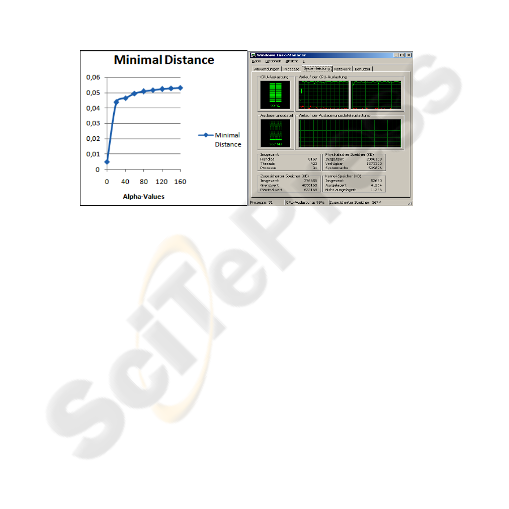
As a measure of the quality of approximation the distance of the “worst-classified”
element to the nearest cut-off was computed. In order to obtain a reference value it
should be mentioned that the optimal margin for arbitrary weights was obtained as
0.0739745 by quadratic programming in [10]. It should also be pointed out that as for
arbitrary weights, cf. [10], the time requirements increased roughly linearly with α,
the maximum time taken (for α = 160) being 29656 msecs. The results obtained are
displayed in diagram 1.
Diagram1 Diagram 2
As may be seen from diagram 1 the quality of approximation to the optimal solution
improves quite fast with increasing α up to about 40. Thereafter, however, only slow
progress is made. Nevertheless, for practical purposes this approximation may be
quite acceptable. In view of the additional condition needed to guarantee convergence
it should also be pointed out that in all other experiments, see also 3.4 below, the
algorithm gave very good results by increasing the distance of the worst classified
element from the nearest cutoff by a factor of about 4 to 10.
3.4 Implementation with Concurrent Java Programming
In view of the fact that multi-processor machines are beginning to dominate the PC
market it seems important that the algorithm presented can be parallelized by
exploiting concurrent Java programming. This is essentially achieved by splitting the
main loop of the algorithm into n (= number of processors) loops of roughly equal
size and assigning them to separate Java worker threads. In each thread then the
required minima are computed separately. The results are passed to the main thread
which computes the overall minimum and updates the weights and cutoffs
accordingly. Thereafter the updated values are passed to the worker threads and the
217

process is repeated. The required synchronization can be obtained by using the Java
classes “BlockingQueue” and “CountDownLatch”, cf.
http://java.sun.com/javase/6/docs/api/java/util/concurrent/BlockingQueue.html
and for the latter class
http://java.sun.com/javase/6/docs/api/java/util/concurrent/CountDownLatch.html.
The authors of the present paper conducted a preliminary test with a dual core
machine that showed that the Java virtual machine splits the work between the two
processors rather nicely if the loop is sufficiently large, see diagram 2 above.
In fact with roughly 12 000 data sets (divided into two preference classes with binary
attribute values only; sufficiently many data encompassing more preference classes
could unfortunately not be obtained) the speed up compared with the ordinary
program version apeared to be close to 100% so that very little administrative
overhead was incurred (incidentally: The total CPU time turned out to be in the order
of three minutes which is surprisingly small). However, a test with a small number of
data even lead to an increase in CPU time, since evidently the administrative
overhead became too large. Nevertheless in practical situations often large data sets
prevail. In view of this fact and because a realization of the dual (kernel) version
would definitely lead to large CPU times (preliminary tests indicate CPU times of
several hours even for quadratic polynomial kernels), the parallelization should be
extremely helpful. The precise variation of the required overhead with the number of
processors is still the subject of ongoing research. Further details will be reported
elsewhere.
4 Conclusion and Outlook
A new large margin ranking algorithm producing positive weights only and thus
removing a potential consistency problem has been presented. Encouraging
experimental evidence has been obtained using “real life” data from a financial
institution. In contrast to the wide margin ranking algorithm described in [20] it can
be implemented with a surprisingly compact Java encoding. This is due to the fact
that it can be seen as an extension of classical perceptron learning. Moreover the
algorithm allows easy parallelization.
On the other hand, of course, it gives only an approximate solution and also needs an
additional condition to guarantee convergence, which may, however, as indicated by
the experimental results, be quite satisfactory for practical applications. In addition
the algorithm works for separable sets only. However, it is intended to combine it
with a modified version of the pocket algorithm, cf.[11], by applying it to those data
sets only that are correctly separated. This seems attractive since that way certain
approximations inherent to the soft margin support vector machine as utilized in [20]
are avoided.
Finally a few comments on related algorithms seem in order. The large margin
algorithm in [20] has been briefly mentioned already. The ranking algorithms in [5]
and [13] appear inferior from the results given in [20]. In [26] large margin
perceptron learning was introduced for the pocket algorithm. However, in spite of
reasonable experimental evidence, the theoretical basis appears slightly shaky, for
details see e.g. the conclusion in [9]. The ranking algorithm in [22] (soft margin
218

version) appears to contain a gap since the monotonicity condition for the cut-offs
seems to be neglected. Moreover an additional vector is ignored without explaining
the consequences. In short then the algorithm closest to the one presented here seems
to appear in [20]. Of course, it has been tested in a completely different context and
an objective comparison concerning the banking application envisaged here is still
outstanding. Moreover none of these algorithms appear to deal with the potetntial
consistency problem discussed in 3.2.
References
1. Banking Committee on Banking Supervision: International Convergence of Capital
Measurements and Capital Standards, A Revised Framework, Bank for International
Settlements, http://www.bis.org/publ/bcbs118.pdf, April 18
th
, 2006
2. Bishop,C.M.: Neural Networks for Pattern Recognition. OUP, (1998)
3. Block, H.D.; Levin, S.A.: On the Boundedness of an Iterative Procedure for Solving a
System of Linear Inequalities. Proc. AMS, (1970)
4. Cover, T.M.: Geometrical and Statistical Properties of Systems of Linear Inequalities with
Applications in Pattern Recognition. IEEE Trans. on Electronic Computers, Vol. 14, (1965)
5. Crammer, K.; Singer, Y.: Pranking with Ranking, NIPS, (2001)
6. Episcopos, A.; Pericli, A.; Hu, J.: Commercial Mortgage Default: A Comparison of the
Logistic Model with Artificial Neural Networks. Proceedings of the 3
rd
Internl .Conference
on Neural Networks in the Capital Markets, London, England, (1995)
7. Falkowski, B.-J.: Lernender Klassifikator, Offenlegungsschrift DE 101 14874 A1,
Deutsches Patent- und Markenamt, München, (Learning Classifier, Patent Number DE 101
14874 A1, German Patent Office, Munich) (2002)
8. Falkowski, B.-J.: On a Ranking Problem Associated with Basel II. Journal of Information
and Knowledge Management, Vol. 5, No. 4, (2006), invited article.
9. Falkowski, B.-J.: A Note on a Large Margin Perceptron Algorithm, Information
Technology and Control, Vol. 35, No. 3 A, (2006)
10. B.-J. Falkowski; M. Appelt; C. Finger; S. Koch; H. van der Linde: Scoring Systems and
Large Margin Perceptron Ranking. In: Proceedings of the 18th IRMA Conference, Vol. 2,
Ed. Mehdi Khosrow-Pour, IGI Publish. Hershey PA USA, (2007)
11. Gallant, S.I.: Perceptron-based Learning Algorithms. IEEE Transactions on Neural
Networks, Vol. I, No. 2, (1990)
12. Hand, D.J.; Henley, W.E.: Statistical Classification Methods in Consumer Credit Scoring: a
Review. Journal of the Royal Statistical Society, Series A, 160, Part 3, (1997)
13. Herbrich, R.; Graepel, T.; Obermayer, K.: Large Margin Rank Boundaries for Ordinal
Regression. In: Advances in Large Margin Classifiers (Eds. Smola, A.J.; Bartlett, P.;
Schölkopf, B.; Schuurmans, D.), MIT Press, Neural Information Processing Series, (2000)
14. Krauth, W.; Mezard, M.: Learning Algorithms with Optimal Stability in Neural Networks.
J. Phys. A: Math. Gen. 20, (1987)
15. Mathieson, M.: Ordinal Models for Neural Networks. Neural Networks in Financial
Engineering, Proceedings of the 3
rd
International Conference on Neural Networks in the
Capital Markets, World Scientific, (1996)
16. Minsky, M.L.; Papert, S.: Perceptrons. MIT Press, (Expanded Edition 1990)
17. Müller, M.; Härdle, W.: Exploring Credit Data. In: Bol, G.; Nakhneizadeh, G.; Racher,
S.T.; Ridder, T.; Vollmer, K.-H. (Eds.): Credit Risk-Measurement, Evaluation, and
Management, Physica-Verlag, (2003)
18. Muselli, M.: On Convergence Properties of Pocket Algorithm. IEEE Trans. on Neural
Networks, 8 (3), 1997
219

19. Shadbolt, J.; Taylor, J.G.(Eds.): Neural Networks and the Financial Markets. Springer-
Verlag, (2002)
20. Shashua, A.; Levin, A.: Taxonomy of Large Margin Principle Algorithms for Ordinal
Regression Problems. Tech. Report 2002-39, Leibniz Center for Research, School of
Comp. Science and Eng., the Hebrew University of Jerusalem, (2002)
21. Shashua, A.; Levin, A.:Ranking with Large Margin Principle: Two Approaches, NIPS 14,
(2003)
22. Shawe-Taylor, J.; Cristianini, N.: Kernel Methods for Pattern Analysis. Cambridge
University Press, (2004)
23. Thomas, L.C.: A Survey of Credit and Behavioural Scoring: Forecasting Financial Risk of
Lending to Consumers. Internl. Journal of Forecasting, 16, (2000)
24. Vapnik, V.N.: Statistical Learning Theory. John Wiley & Sons, (1998)
25. Wong, S.K.M.; Ziarko, W.; Wong, P.C.N.: Generalized Vector Space Model in Information
Retrieval. Proceedings of the 8
th
ACM SIGIR Conference on Research and Development in
Information Retrieval, USA, (1985)
26. Xu, J.; Zhang, X.; Li, Y.: Large Margin Kernel Pocket Algorithm. In: Proceedings of the
International Joint Conference on Neural Networks 2001, IJCNN’01, Vol. 2. New York:
IEEE, (2001)
Appendix
Convergence Theorem
For simplicity here the following problem is considered (the convergence theorem for
the algorithm given in 3.4 may then be deduced by applying the results of section 2):
Given sample vectors (patterns) x
1
, x
2
, …, x
p
∈ Ζ
n
find a vector w* having positive
entries only such that. <w*, x
j
> ≥ α for j= 1,2, …, p and a fixed constant α > 0.
Assume throughout that such a vector exists with ||w*|| = α /Δ
opt
, where Δ
opt
denotes
the maximal separation of the samples from zero.
Then consider the following algorithm
Set w
0
:= 0 and
w
t+1
:= w
t
+ x
j(t)
if < w
t
, x
j(t)
> < α,
where x
j(t)
is defined by
min{min
1≤k≤p
< w
t
, x
k
>, min
1≤l≤n
< w
t
, e
l
>} if min
1≤l≤n
< w
t
, e
l
> ≤ 0
x
j(t)
:=
min
1≤k≤p
< w
t
, x
k
>, otherwise.
General Convergence Properties
After M updates according to this rule suppose that pattern x
j
has been visited m
j
times and that the j-th unit vector e
j
has been visited λ
j
times where
p
1
M
j
j=
∑
= M
1
and = Λ; M
1
+ Λ = M.
220

Further assume that there exists a w* with positive entries such that
(i) <w*, x
j
> ≥ α for j= 1,2, …, p
(ii) <w*, e
j
> > 0 for j= 1,2, …, n
(iii) ||w*|| = α /Δ
opt
Then the following bounds for <w*, w
M
> are obtained:
Lower bound: <w*, w
M
> ≥ M
1
* α + Λ*min
1
≤
k≤n
w*[k] ≥ M* α
1
(1)
where α
1
:= min{ α, min
1≤k≤n
w*[k]}
Upper bound: ||w
M
||
2
- ||w
M-1
||
2
= 2<w
m-1
, x
j(m-1)
> + || x
j(m-1)
||
2
≤ 2α + B say, where
B:=max{max
1≤k≤p
|| x
k
||
2
,1}
Hence ||w
M
|| ≤ {M(2 α +B)}
1/2
.
And thus by the Cauchy-Schwartz inequality
<w*, w
M
> ≤ ||w*||{M(2α +B)}
1/2
(2)
(1) and (2) together imply convergence since M
1/2
≤ ||w*||(2α +B)
1/2
/α
1
.
Optimal Margin of Separation
In order to show that the algorithm gives the optimal margin of separation as α → ∞
one needs an additional assumption (note that in view of the experimental results
given above this does not seem too restrictive), namely additional assumption
: α = α
1
.
As in [14] decompose w
t
as w
t
= a(t)w* + k
t
where <k
t
,w*> = 0.
Argue as above but reason separately for w* and k
t
by decomposing x
j(t)
accordingly.
First note that a(t) = <w
t
, w*>/||w*||
2
and hence that a(t) > 0 for t ≥ 1 because of
assumptions (i) and (ii) for ||w*||.
Further note that x
j(t)
always has a negative projection on k
t
, i.e. < k
t
, x
j(t)
> < 0, since
this has been shown for x
j(t)
= x
k
for some k satisfying 1 ≤ k ≤ p in [9],[14], and for
x
j(t)
= e
l
for some l satisfying 1 ≤ l ≤ n it follows since then <w
t
, e
l
> = a(t)<w*, e
l
> +
<k
t
, e
l
> ≤ 0, where a(t)<w*, e
l
> > 0 because of the positivity of a(t) and property (ii)
of ||w*||.
Moreover w
t+1
= w
t
+ x
j(t)
=
[a(t) + < x
j(t)
, w*>/||w*||
2
] w* + [1 + < x
j(t)
, k
t
>/|| k
t
||
2
] k
t
whence ||k
t
||
2
- ||k
t-1
||
2
= 2< x
j(t-1)
, k
t-1
> + || x
j(t-1)
||
2
≤ B.
Thus ||k
t
||
2
≤ t*B (3)
If learning stops after M steps then a(M-1) can be bounded as follows
<w
M-1
, x
j(M-1)
> = a(M-1) <w*, x
j(M-1)
> + <k
M-1
, x
j(M-1)
> < α.
Hence, using the additional assumption and property (i) of w* one obtains
a(M-1) < [α + |<k
M-1
, x
j(M-1)
> |]/ α.
From this it follows that
a(M-1) ≤ [α + ||k
M-1
||*|| x
j(M-1)
||]/ α ≤ [ α + (M-1)
1/2
B]/ α (4)
A bound on a(M) is then obtained via
a(M) – a(M-1) = <w
M
– w
M-1
, w*>/||w*||
2
= |< x
j(M-1)
, w*>|/||w*||
2
≤ B
1/2
/||w*||
221

= B
1/2
Δ
opt
/α (5)
Hence, using (4) and (5), a(M) ≤ [α + (M-1)
1/2
B]/α + B
1/2
Δ
opt
/α (6)
Using (6) gives
||w
M
|| = a(M)||w*|| + ||k
M
|| ≤ {[α + (M-1)
1/2
B]/α + B
1/2
Δ
opt
/α}||w*|| + MB
1/2
= ||w*||{[ α + (M-1)
1/2
B]/c + B
1/2
Δ
opt
/α + (Δ
opt
/α) MB
1/2
} 7)
Finally from (7) one obtains α /Δ
opt
≤ α /Δ
α
≤ ||w
M
|| → ||w*|| = α /Δ
opt
as α → ∞ since
M grows at most linearly with α.
222
