
A Colour Space Selection Scheme dedicated to
Information Retrieval Tasks
Romain Raveaux, Jean-Christophe Burie and Jean-Marc Ogier
L3I Laboratory – University of La Rochelle, France
Abstract. The choice of a relevant colour space is a crucial step when dealing
with image processing tasks (segmentation, graphic recognition…). From this
fact, we address in a generic way the following question: What is the best
representation space for a computational task on a given image? In this article, a
colour space selection system is proposed. From a RGB image, each pixel is
projected into a vector composed of 25 colour primaries. This vector is then
reduced to a Hybrid Colour Space made up of the three most significant colour
primaries. Hence, the paradigm is based on two principles, feature selection
methods and the assessment of a representation model. The quality of a colour
space is evaluated according to its capability to make colour homogenous and
consequently to increase the data separability. Our framework brings an answer
about the choice of a meaningful representation space dedicated to image
processing applications which rely on colour information. Standard colour
spaces are not well designed to process specific images (ie. Medical images,
image of documents) so a real need has come up for a dedicated colour model.
1 Introduction
Colour representation is the basement of all colour image processing applications. In
fact, many colour spaces were developed for graphics and digital image processing
such as Red, Green, Blue (RGB) and Hue, Saturation. Intensity (HSI). Nevertheless, it
is obvious that the performance of any colour-dependent system is highly influenced
by the colour model it uses. The quality of a colour model is defined by its capacity to
correctly distinct colour between them while being robust to variations inside a given
chromatic cluster such as light changes. In term of datamining, this problem can be
addressed as maximizing the distance inter-classes while minimizing the distance
intra-class. These two criteria seem to be conflicting, which represents a real
challenge to any colour representation scheme. Many information retrieval
applications would benefit for a better representation space. The paper is organized as
follows: In the second section, the question of finding the best colour space is
introduced with a review of the related work. Thirdly, the global concept is described
explaining the methodology of our contribution. Then, the fourth section presents the
feature selection methods in use in this paper. The fifth section presents experimental
results on colour classification according different colour models, in addition a
Raveaux R., Burie J. and Ogier J. (2008).
A Colour Space Selection Scheme dedicated to Information Retrieval Tasks.
In Proceedings of the 8th International Workshop on Pattern Recognition in Information Systems, pages 123-134
Copyright
c
SciTePress
comparative study on cadastral map segmentation is presented. Finally, a conclusion
is given and future works are brought in section 5.
2 Related Work
In this section, reference to previous works on this field of science is done starting by
classical colour spaces to finally present the selection of colour components.
2.1 Standard Colour Spaces
Most of acquisition devices, such as digital cameras or scanners, process signals in the
RGB format. This is why RGB space is widely used in the applications of image
processing. The R primary in RGB corresponds to the amount of the physical
reflected light in the red band. However, RGB representation has several drawbacks
that decrease the performance of the systems which depend on it. RGB space is not
uniform; the relative distances between colours do not reflect the perceptual
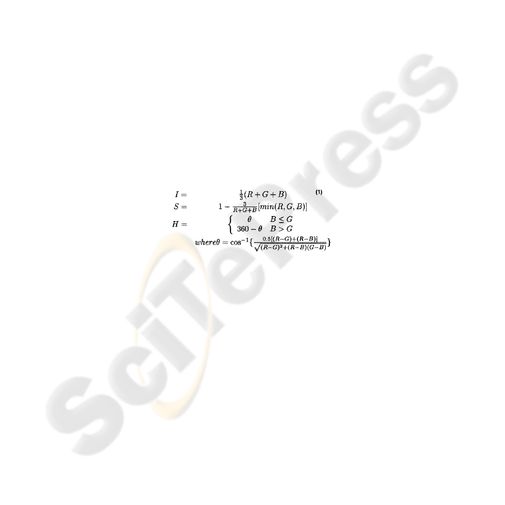
differences. Therefore, HSI space has been developed as a closer representation to the
human perception system, which can easily interpret the primaries of this space. In
HSI space, the dominant wavelength of colour is represented by the hue component.
The purity of colour is represented by the saturation component. Finally, the darkness
or the lightness of colour is determined by the intensity component. Eq.(1) shows the
transformation between RGB and HSI spaces [1].
Although the HSI space is suitable for lots of applications based on colour images
analysis, this colour space presents some problems. For example, there are non-
avoidable singularities in the transformation from RGB to HSI, as shown in Eq.(1).
The XYZ colour space developed by the International Commission on Illumination
(CIE) in 1931 [2] is based on direct measurements of the human eye, and serves as the
basis from which many other colour spaces are defined. The YUV colour is used in
the PAL system of colour encoding in analogical video, which is part of television
standards. The YUV model defines a colour space in terms of one luminance and two
chrominance components. Another alternative of YUV is the YIQ which is used in
the NTSC TV standard. On the other hand, Ohta, Kanade, and Sakai [3] have selected
a set of "effective" colour features after analyzing 100 different colour features which
have been used in segmenting eight kinds of colour images. Those selected colour
features are usually names as I1I2I3 colour model. XYZ, YUV and I1I2I3 are non-
uniform colour spaces; therefore CIE has recommended CIE-Lab and CIE-Luv as
uniform colour spaces, as they are non-linear transformation of RGB space [4].
124

2.2 Hybrid Colour Spaces
Recently, the question of finding the best colour representation has generated a rich
literature. In [5], a standard colour space is picked-up specifically for a given image
however the process involved does not consider the possibility to combine colour
components from several spaces. To solve this problem, in [6], dominant features
from different colour spaces are selected to construct a DHCS (Decorrelated Hybrid
Colour Space). A Principal Component Analysis (PCA) is performed from the
covariance matrix composed with the total number of the candidate primaries. The 3
most significant axis are selected to reduce rate of correlation between colour
components. On the other hand, our approach aims to maximise one criterion which is
the colour recognition rate (Eq 2) while others methods [7] try to compromise indices
(compacity and classes dispersion) in order to assess the suitability of a colour model.
2) (Eq
PixelsColour #
PixelsColour ClassifiedCorrectly #
Rec =
These indices represent two competitive constraints, in other word, two conflicting
objectives, the improvement of one of them leads to the deterioration of the other.
Each image is like no other, so it deserves a dedicated colour representation. We
believe, it is hardly possible to generalize the colour pixel distribution for a given
image set. So it seems unlikely feasible to apply the same colour space on all the
images contained in a database. Each image must be considered independently. in [8],
soccer players are classified, according to their colour information, using supervised
learning techniques, this training stage supposed to dispose of the user ground truth
which is not often the case, and limit the flexibility of the system. Our framework is
generic since it relies on a parsimonious use of machine learning algorithms.
Furthermore, we handle different feature selection methods, we take advantages of
their different ways to reach a single goal.
3 Methodology
The main architecture of our framework is presented in figure 1. It starts from an
RGB image where each pixel is projected into nine standard colour spaces in order to
build a vector composed of 25 colour components. Let C be a set of colour
components.
{} { }
*,...*,*,,3,2,1,,,
1
vuLIIIBGRCC
N
i
i
==
=
with Card(C)=25. From
this point, pixels represent a raw database, an Expectation Maximization (EM)
clutering algorithm is performed on those raw data in order to label them. Each
feature vector is tagged with a label representing the colour cluster it belongs to.
125
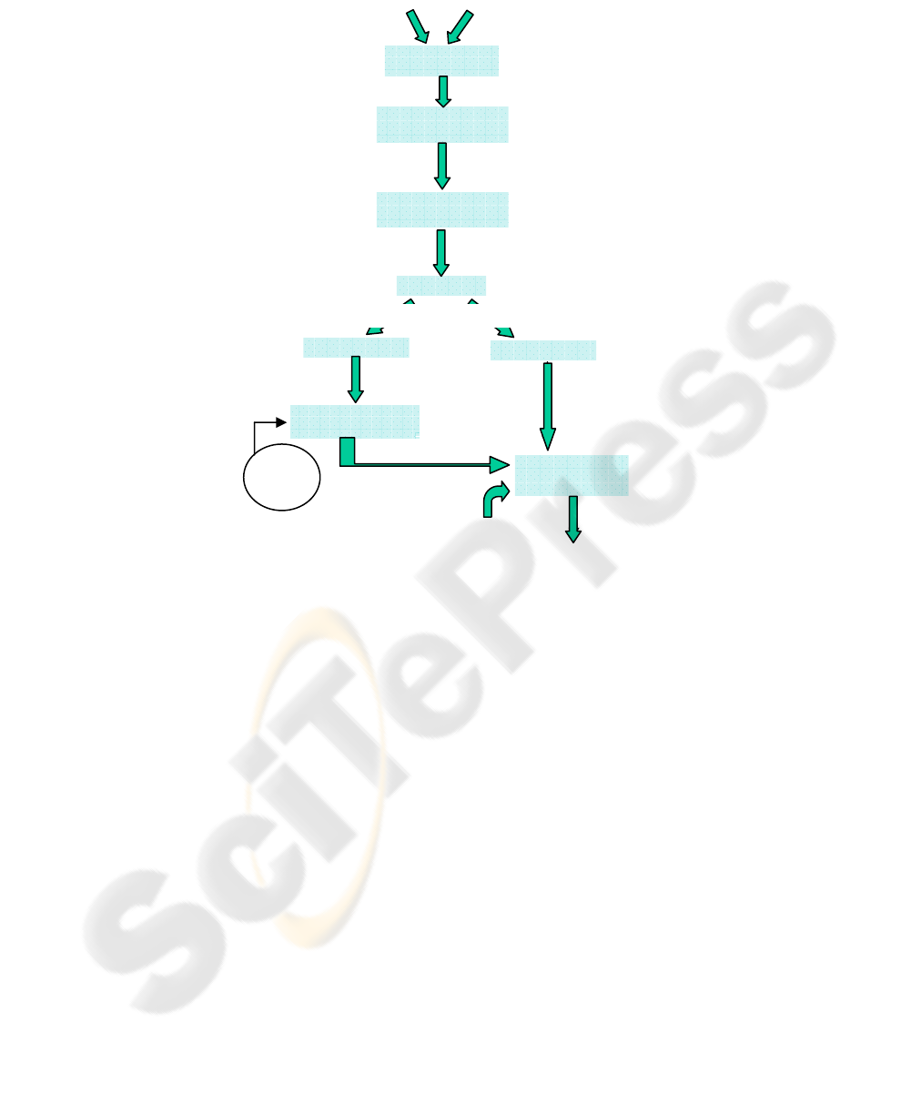
Fig. 1. A framework for colour space selection.
4 Feature Selection Methods
The selection of features is a very active area in recent years, especially in the context
of data mining. Indeed, the data mining in very large databases is becoming a critical
issue for applications such as image processing, finance, etc. It is important to
summarize and intelligently retrieve the "knowledge" from raw data. The data mining
is an area based on statistics, machine learning and the theory of databases. The
variable selection plays an important role in data mining especially in the preparation
of data prior to processing. Indeed, the interests of the variable selection are as
follows:
- When the number of variables is just too great learning algorithm can not finish in a
good time. The selection reduces the dimension of feature space.
- In terms of artificial intelligence, creating a classifier returns to create a model for
the data. However, a legitimate expectation for a model is to be as simple as possible
(principle of Occam's razor [9]).
Sub Sampling
RGB Image Illuminant
Clustering : EM
Projection in Standard
Spaces
Features selection
Evaluation
1-NN Classification
Pixels In RGB Space
Pixels projected
in 9 spaces
1 pixel = 1 vector with 25
colour components
A set of data
Training set
Test set
Sets of selected features.
Hybrid Spaces
Confusion
rate for each
space
Labeled data
bases
-9 Standard spaces :
(L*a*b*,I1I2I3,..)
K significant clusters are found and split into 2 labeled DB
Labeled data
bases
- CFS
- Genetic Search
- PCA Space
- One R
126
Reducing the size of the space feature allows us to reduce the number of required
parameters for the description of this model also avoiding the phenomenon of over-
fitting and emphasizing the synthesize information.
- It improves the performance of the classification, its speed and power of
generalization.
- It increases the data understanding: a better view of what are the processes that give
rise to them. This selection consists of:
Æ The elimination of independent variables of the class,
Æ The elimination of redundant variables.
4.1 Global Concept
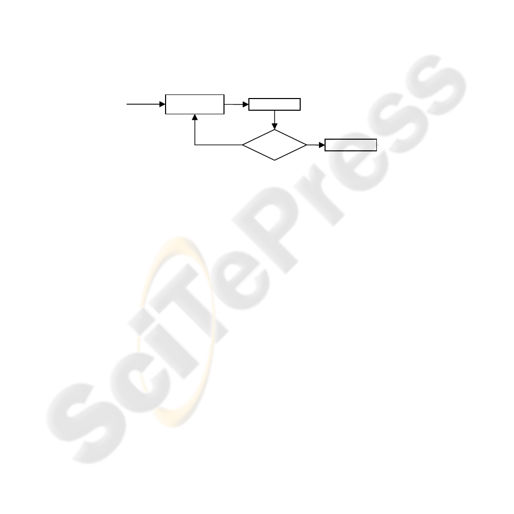
A general structure for selecting features can be offered in the way of figure 2 ([10]).
Up to a certain criterion to be satisfied, sub sets are generated in browsing the feature
space.
Fig. 2. Feature selection architecture.
The subsets generation is a searching process in the subset space of cardinality 2
N
with N the number of features. All classical searching algorithms can be applied to
that problem. For instance [11] proposes the methods forward addition and backward
elimination (deletion), [12] and [13] have made a good use of evolutionary
algorithms.
4.2 Searching Algorithm and Evaluation
Existing feature selection methods for machine learning typically fall into two broad
categories—those which evaluate the worth of features using the learning algorithm
that is to ultimately be applied to the data, and those which evaluate the worth of
features by using heuristics based on general characteristics of the data. The former
are referred to as wrappers and the latter filters.
1. Wrappers use classification algorithm to evaluate the pertinence of a given sub set
of variables. Genetic Algorithms (GA) dedicated to colour space selection are
wrappers based on heuristics. GA for Colour Space(GACS) encodes its individuals as
vectors limited to three components specifically adapted to the colour representation
[14]. 2. Filters are completely independent from the classification stage. They are
based on statistical concepts: entropy, coherence… A good feature subset is one that
contains feature highly correlated with predictive of the class and yet uncorrelated
with the others [10].
Sub set generation
Evaluation
Validation
Stopping criterion
Starting
Set
no
yes
127

The Wrappers. Although conceptually more simple than filters, wrappers were
introduced more recently by John, and Kohavi Pfleger in 1994. Their principle is to
generate subsets candidates and to evaluate them thanks to a classification algorithm.
The score or merit will be a combination of a trade-off between the number of
variables eliminated, and the classification rate on a test file. Thus, the “assessment”
stage of the selection cycle is made by a call to the classification algorithm. In fact,
the classification algorithm is called several times for each evaluation because a
cross-validation is frequently used. By its very intuitive principle, this method
generates subsets well suited to the classification algorithm. Recognition rates are
high since the selection takes into account the intrinsic bias of data. Another
advantage is its conceptual simplicity: there is no need to understand how the
induction is affected by the selection of variables, it is sufficient to generate and test.
However, there are three reasons that the wrappers are not a perfect solution. First,
they do not really have theoretical justification for the selection and they do not allow
us to understand the conditional dependencies that may exist between the variables.
On the other hand, the selection process is specific to a particular classification
algorithm and find subsets are not necessarily valid if you change the method of
induction. Finally, and this is the main defect of the method, the calculations quickly
become quite long when the number of variable grows up.
The Filters. Filters don’t have the defects of wrappers. They are much faster, they are
based on more theoretical considerations, it allows a better understanding to the
dependency relationships between variables. But, as they do not take into account the
biases of the classification algorithm, the subsets of variables generated give a lower
recognition rate. To give a score to a subset, the first solution is to give a score to each
variable independently of the others and to do the sum of those scores [OneR
Selection]. The alternative is to evaluate a subset as a whole [12]. We are closer here
learning the Bayesian network structure. There is an intermediary between ranking
and feature subset ranking based on an idea of Ghiselli and used with good results in
the context of the CFS (correlation based feature selection) by Mr. Hall [10]. The
score of a subset is constructed based on correlations variable-class and correlations
variable-variable ( Eq 3):
Equation. 3. Correlation score associated to each feature in CFS method
ii
zi
zc
rkkk
rk
r
)1( −+
=
Where
zc
r is the correlation between the summed components and the outside variable
(a given colour cluster – a class), k is the number of components,
zi
r is the average of
the correlations between the components and the outside variable, and
ii
r is the
average inter-correlation between components
This equation express that the merit of a given subset increase if the variables are
highly correlated with the class and it decrease if features are highly correlated
between each others. The idea is to state that a “good” subset is composed of
variables highly correlated with the class (to discard independent variables) and
loosely correlated between them/features (to avoid redundant components). It is an
128
approximation since it only takes into account the interactions of order 1. The
correlation or dependency between two variables can be defined in several ways.
Using the statistical correlation coefficient is too restrictive because it only captures
the linear dependence. However, one can use a test of independence as the statistical
test of
2
χ
. It is also possible to combine wrapper and filter as presented in [13]
4.3 Stopping Criterion
The stopping criterion may take various forms: a computation time, a number of
generations (for a genetic algorithm), a number of selected variables or a heuristic
evaluation of the subset “value”.
Table 1. Selection feature methods in use.
Name Type Evaluation Searching algorithm
CFS
Filter CFS Greedy stepwise
EHD
Filter PCA
*
Ranker
GACS
Wrapper Classification Genetic Algorithm
OneRS
Wrapper Classification Ranker
4.4 Hybrid Colour Space built by Genetic Algorithm. GACS
In Hybrid Colour Space (HCS) context, each individual has to encode a vector, where
each component is an axis of the HCS. We consider a set C of features.
{}
{
}
*,...*,*,,3,2,1,,,
1
vuLIIIBGRCC
N
i
i
==
=
with Card(C)=25. Practically, it is
almost impossible to test all possible combinations, since they have a combinatory
number equal to the factorial of the total number of the candidate primaries, hence,
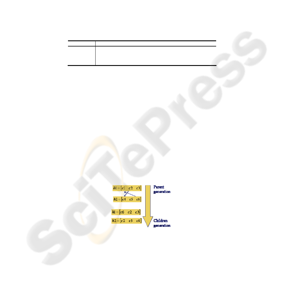
Genetic Algorithm are well suited to get rid off absurd combinations. From now, the
first step is to initialize the population, each individual is made up picking randomly
three elements of C. Concerning cross over operator, two individuals h1 and h2 share
their genetic material, swapping one of their component; fig 3. Finally, to perform
mutation on an individual, one component is selected and replaced at random by an
element of C. Finally, the evaluation phase computes a 1NN classifier based on a
Euclidian metric. A cross-validation system is run on the training base.
Fig. 3. HCS: cross over operator.
129
5 Experiments
5.1 Context
In the idea to assess our system, we perform two evaluation stages. The first one is a
colour classification step to test if the colour representation found by our framework
is interesting in term of colour distinction. The second step is a segmentation phase.
Indeed, a better representation system should give better segmentation results.
5.2 Colour Classification
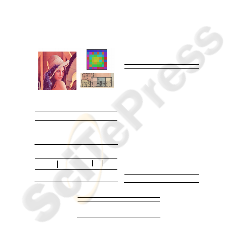
Our approach is applied on three different types of images. A natural scene, an image
of the document and a synthetic image. Each colour space is evaluated on the test
dataset through the use of a 1NN classification step. In table 2, the number of colour
clusters found by the clustering algorithm(EM) is given. Table 4 shows the
components selected by the several feature selection techniques.
Fig. 4. Images in use.
Table 2. Test images description.
Id Image Type # of
clusters
Im1
Lenna Natural Scene 18
Im2
SatSnake Synthetic image,
discriminating
by the saturation
23
Im3
Image of
document
Ancient
Cadastral Map
9
Table 3. Training and Test Databases.
training
X pixels
test
X pixels
IM1 130107 130107
IM2 100951 100951
IM3 110424 110424
Table 4. Hybrid Colour Spaces found on the
Image IM2.
Attributes CFS GACS
DHCS
OneRs
R 0 0 0 0
G 1 0 1 0
B 1 0 0 0
I1 0 0 0 0
I2 1 0 0 0
I3 0 0 0 0
T 1 1 0 1
S 1 1 0 1
I 0 0 0 0
L* 1 0 0 0
a* 1 0 0 0
b* 1 0 0 0
L* 0 0 0 0
u* 1 1 0 0
v* 1 0 0 0
A 0 0 0 0
C1 1 0 0 0
C2 1 0 0 0
X 0 0 0 0
Y 0 0 1 0
Z 1 0 1 0
Y 0 0 0 0
I 1 0 0 1
Q 1 0 0 0
Y 0 0 0 0
U 1 0 0 0
V 0 0 0 0
# of
attributes
16 3 3 3
Table 5. Number of selected features.
# of selected attributes
CFS GACS EHD OneRS
IM1 16 3 3 3
IM2 16 3 3 3
IM3 12 3 3 3
130

Table 6. Confusion rate on Image 1.
IM1
Colour
Spaces
Error ColourSpaces Error
RGB
0.3608
TSI
0.3917
I1I2I3
0.3814
La*b*
0.4329
XYZ
0.3814
L*u*v*
0.4948
YIQ
0.4742
DHCS
0.3917
YUV
0.3195
CFS
0.0615
AC1C2
0.4123
GACS 0.2680
PCA
0.3711
OnRS
0.3608
Table 7. Confusion rate on Image 2.
IM2
Colour Spaces Error Colour Spaces Error
RGB
0.22
TSI
0.51
I1I2I3
0.24
La*b*
0.41
XYZ
0.23
L*u*v*
0.35
YIQ
0.43
DHCS
0.39
YUV
0.35
CFS
0.14
AC1C2
0.29
GACS 0.19
OnRS
0.39
PCA
0.35
Table 8. Confusion rate on Image 3.
IM3
Colour Spaces Error Colour Spaces Error
RGB
0.5444
TSI
0.3666
I1I2I3
0.2222
La*b*
0.2666
XYZ
0.5777
L*u*v*
0.3333
YIQ
0.3111
DHCS
0.36
YUV
0.3777
CFS
0.0333
AC1C2
0.3
GACS 0.1888
OnRS
0.4111
PCA
0.2444
5.3 Application to Segmentation and Evaluation
Once the source image is transferred into a suitable hybrid colour space, an edge
detection algorithm is processed. This contour image is generated thanks to a vectorial
gradient according to the following formalism. The gradient or multi-component
gradient takes into account the vectorial nature of a given image considering its
representation space (RGB for example or in our case hybrid colour space). The
vectorial gradient is calculated from all components seeking direction for which
131

variations are the highest. This is done through maximization of a distance criterion
according to the L2 metric, characterizing the vectorial difference in a given colour
space. The approaches proposed by DiZenzo[7] first, and then by Lee and Cok under
a different formalism are methods that determine multi-components contours by
calculating a colour gradient from the marginal gradients.
Given 2 neighbour pixels P and Q characterizing by their colour attribute A, the
colour variation is given by the following equation:
)()(),( PAQAQPA
−
=
Δ
The pixels P and Q are neighbours, the variation
A
Δ
can be calculated for the
infinitesimal gap: dp = (dx, dy)
dy
y
A
dx
x
A
dA
∂
∂
+
∂
∂
=
This differential is a distance between pixels P and Q. The square of the distance is
given by the expression below:
()()()
()()()
2
3
2
2
2
1
332211
2
3
2
2
2
1
22
2
2
2
2
2
2
2
e
y
e
y
e
y
e
y
e
x
e
y
e
x
e
y
e
x
e
x
e
x
e
x
GGGc
GGGGGGb
GGGa
cdybdxdyadx
dy
y
A
dxdy
y
A
x
A
dx
x
A
dA
++=
++=
++=
++=
⎟
⎟
⎠
⎞
⎜
⎜
⎝
⎛
∂
∂
+
∂
∂
∂
∂
+
⎟
⎠
⎞
⎜
⎝
⎛
∂
∂
=
Where, E can be seen as a set of colour components representing the three primaries
of the hybrid colour model. And where
m
n
G can be expressed as the marginal
gradient in the direction
n for the m
th
colour components of the set E.
The calculation of gradient vector requires the computation at each site (x, y): the
slope direction of A and the norm of the vectorial gradient. This is done by searching
the extrema of the quadratic form above that coincide with the eigen values of the
matrix M.
⎟
⎟
⎠
⎞
⎜
⎜
⎝
⎛
=
cb
ba
M
The eigen values of M are:
⎟
⎠
⎞
⎜
⎝
⎛
+−±+=
±
22
4)(5.0 bcaba
λ
Finally the contour force for each pixel (x,y) is given by the following relation:
−+
−=
λλ
),( yxEdge
These edge values are filtered using a two class classifier based on an entropy
principle in order to get rid off low gradient values. At the end of this clustering stage
a binary image is generated. This image will be called as contour image through the
rest of this paper. Finally, regions are extracted by finding the white areas outlined by
black edges. In order to compare the results between the segmented image generated
by the computer and the user defined ground truth, the Vinet criterion[15] is chosen
[Tab 9].
132

Table 9: Segmentation evaluation on Hybrid Colour Space.
Dizenzo Segmentation
Colour Cadastral maps
# of regions Vinet
criterion
RGB image 1714 0.5703
HCS found by GACS 1596 0.5821
Another way to assess a segmentation process is to compute the Levin and Nazif (LN)
criterion. It takes into parameters the segmented image and the original image and
returns a score, the higher the better. This comparison is carried out on a set of 50
maps. Levin and Nazif criterion[15] is the union of two principles, the disparity intra
and inter regions.
Table 10 : Comparison HCS and RGB spaces on a segmentation process using LN criterion.
Dizenzo Segmentation
Colour Cadastral maps
LN Criterion on 50 images
Average Std deviation
RGB 0.4770375 0.005396543
HCS 0.480325 0.007211647
5.4 Analyze
The quality of a colour model is judged by two decisive factors: "Robustness" and
"Distinction". The robustness of the colour representation is an indication of the
sensitivity of colour values to illumination and brightness variations. The
“Distinction” capacity of a colour model is directly linked to its capacity to separate
one colour to the others.
The colour space minimizing the error rate classification is the most discriminating
space for a given image [Tab 6,7,8]. The space generating the least mistake will be
retained to continue treatments on the image. The chosen space is minimizing the
distance intra-class, within the same unit chromatic while maximizing the distance
inter-classes. Such properties are helpful in post-processing stages such as
segmentation, or graphics recognition. Thanks to a well suited colour model, the
number of regions has been reduced by 118 decreasing the over-segmentation
problem, moreover, the Vinet criterion has been improved by 2% getting closer to
user ground truth. At the same time, the LN criterion results lead to the same
conclusion, showing that the contrast inter regions and the homogeneity intra-region
are slightly better in HCS than in the RGB case. These results are encouraging and
they demonstrate how important it is to choose a “good” colour model.
6 Conclusions
In this paper, we have presented a colour space selection framework. Our contribution
focuses on a “all-in-one” system to find a suitable colour space. Our tool can be seen
as a pre-process to any colour information retrieval application (Segmentation,
graphic recognition …). Our approach aims to maximise one criterion which is the
colour recognition rate to unleash the colour information. Each image is like no other,
133

so a dedicated colour representation is required. We believe, it is hardly possible to
model a unique colour space from a given image set and then to apply this “mean
model” individually, that’s why our method computes independently a dedicated
model to each image. Our framework relies on a wise use of different feature
selection methods in order to take advantages of their diverse ways to reach a single
goal. Finally, Hybrid Colour Spaces are particularly well suited while dealing with
very specific images, such as medical images, images of documents where CIE spaces
are not particularly well designed. We believe that much colour image software would
get profit to the use of an adapted colour space.
References
1. J. M. Tenenbaum, T. D. Garvey, S.Weyl, and H. C.Wolf. An interactive facility for scene
analysis research. Technical Report 87, Adapted Intelligent Center, Stanford Research
Institute, Menlo Park, CA, 1974.
2. http://www.cie.co.at/cie/index.html.
3. Y. I. Ohta, T. Kanade, and T. Sakai. Colour information for region segmentation. Computer
Graphics and Image Processing, 13:222-241, 1980.
4. H. Palus. Colour spaces. In S.J. Sangwine and R.E.N. Home, editors, The Colour Image
Processing Handbook, pages 67-90. Chapman & Hall, Cambridge, Great Britain, 1998.
5. L. Busin, N. Vandenbroucke, L. Macaire et J.-G. Postaire, Color space selection for
unsupervised color image segmentation by histogram multithresholding, dans Proceedings
of the 11th International Conference on Image Processing (ICIP'04), Singapoure, pp. 203-
206, Octobre 2004 -
6. J. D. Rugna, P. Colantoni, and N. Boukala, “Hybrid color spaces applied to image
database," vol. 5304, pp. 254{264, Electronic Imaging, SPIE, 2004.
7. N. Vandenbroucke, L. Macaire, and J.G. Postaire. Color pixels classification in an hybrid
color space. In Proceedings of the IEEE International Conference on Image Processing -
ICIP'98, volume 1, pages 176-180, Chicago, 1998.
8. N. Vandenbroucke, L. Macaire, and J. G. Postaire. Color image segmentation by pixel
classification in an adapted hybrid color space: application to soccer image analysis.
Computer Vision and Image Understanding, 90(2):190-216, 2003.
9. Anselm Blumer, Andrzej Ehrenfeucht, David Haussler, and Manfred K.Warmuth. Occam’s
razor. Information Processing Letters, 24(6) :377–380, 1987.
10. M. Hall. Correlation-based feature selection for machine learning, 1998. Thesis IN
Computer Science at the University of Waikato.
11. Daphne Koller and Mehran Sahami. Toward optimal feature selection. In International
Conference on Machine Learning, pages 284–292, 1996.
12. P. Dangauthier. Feature Selection For Self-Supervised Learning, AAAI Spring Symposium
Series, AAAI (American Association for Artificial Intelligence), 445 Burgess Drive, Menlo
Park, California 94025-3442 USA, March 2005
13. Jihoon Yang and Vasant Honavar. Feature subset selection using a genetic algorithm. IEEE
Intelligent Systems, 13 :44–49, 1998.
14. Romain Raveaux, Jean-Christophe Burie, Jean-Marc Ogier. A colour document
interpretation: Application to ancient cadastral maps. The 9th International Conference On
Document Analysis(ICDAR 2007).
15. Adaptative evaluation of image segmentation results C. Rosenberger Pattern Recognition,
2006. ICPR 2006. 18th International Conference on Volume 2, Issue , 2006 Page(s):399 -
402 Digital Object Identifier 10.1109/ICPR.2006.214
134
