
RFID based Anti-Counterfeiting Utilizing
Supply Chain Proximity
Ali Dada and Carsten Magerkurth
SAP Research, SAP Research CEC St. Gallen, 9000 St. Gallen, Switzerland
Abstract. This paper discusses a novel RFID-based approach to determine
probabilities of items in a supply chain as being counterfeits based on their
proximity to already identified counterfeits. The central idea is that items
moving close to fakes are more likely to be fakes than items traveling with
genuine items. The required proximity information can be deduced from events
in EPCIS repositories for RFID-tagged items. The paper discusses two
mathematical algorithms for calculating the probabilities and presents the
results of a comparative simulation study. The results are discussed in terms of
conclusions for a future implementation with RFID-tracked supply chains.
1 Introduction
The International Anti-Counterfeiting Coalition
1
estimates that sales of counterfeits
are a $600 billion a year problem that causes losses in revenues, brand damages, and
that can even be hazardous to health and well-being in the case of faked drugs or
faked parts in the airline or car industries [1].
Until the emergence of RFID-based track & trace standards such as EPCglobal
2
,
anti-counterfeiters had to rely on direct authentication measures almost exclusively.
The question of how to authenticate a product was addressed with security features
like holograms, copy detection patterns (CDP), or even cryptographic RFID tags [2,
3]. While these features are generally appropriate for authenticating products and
identifying fakes, the critical issue of how to locate and where to search for potential
counterfeits in the first place can be addressed with transparent supply chains utilizing
EPC Information Services [4] or similar RFID-based tracking mechanisms.
The basic observation and premise is that counterfeits in the domain of fast
moving consumer goods (FMCG) usually enter the supply chains together with
similar counterfeits, for instance in the same container or palette, and that these
counterfeits consequently move together through parts of the supply chain.
Whenever a counterfeit is located by any direct authentication measure, we can
identify other potential counterfeits that were close to the already confirmed
counterfeits at some point in the supply chain.
1
www.iacc.org
2
www.epcglobalinc.org
Dada A. and Magerkurth C. (2008).
RFID based Anti-Counterfeiting Utilizing Supply Chain Proximity.
In Proceedings of the 2nd International Workshop on RFID Technology - Concepts, Applications, Challenges, pages 101-114
DOI: 10.5220/0001742601010114
Copyright
c
SciTePress

With this proximity information about potential counterfeits calculated on data
gathered from RFID-based tracking services, the allocation of anti-counterfeiting
resources to potentially suspicious items is facilitated. This way, resources-
constrained bodies such as customs could direct their resources more efficiently
towards identifying which items to check.
The solution discussed in this article is based on the unique identification of
individual items in the supply chain and the tracking and tracing of these items
including parent-child (aggregation) relations. Information about these relations are
provided as events in EPC Information Services (EPCIS) for RFID tagged items, but
could potentially be gathered through other emerging standards as well. The solution
works by assigning probabilities based on proximity to items known to be counterfeit
or authentic.
2 Supply Chain Proximity
As pointed out in the introduction, the central constituent of the approach discussed in
this paper is that – as long as no specific other knowledge is available – the
probability of an item in a supply chain being counterfeit increases with its proximity
to already identified counterfeits. This assumption is based on the fact that inserting
counterfeits in a licit supply chain is neither always possible at any given time or
position, nor is it cost-efficient for the counterfeiter to equally balance the inclusion of
counterfeits. Hence, an inclusion attack on a licit supply chain will usually involve
multiple items at once, so that the spatial (or temporal) proximity to a counterfeit item
positively affects the probability of an item to be counterfeit as well.
In the domain of RFID-based tracking and tracing of items, we commonly deal
with aggregating and disaggregating events to model the hierarchical realities of
logistics with items moving in cases, pallets, containers, shipments, etc.
Consequently, we also create corresponding data structures that define proximity in
terms of hierarchical relationships as is discussed in section 0.
To determine the likelihood that an item is counterfeit, we assign a fakeness
probability to each item depending on its spatial and temporal proximity to already
verified items. We explain in section 0 two alternative algorithms through which we
calculate the fakeness probabilities, but first we introduce in section 0 the concept of
proximity in a supply chain and the supporting structures.
Item Hierarchy Structures. The fakeness probability algorithms we will introduce
make use of hierarchical structures that denote the temporal and spatial proximity
between items in the supply chain. The structures are generic as they support different
concepts of proximity. For example, proximity between two items can imply their
ownership by the same supply chain partner at a certain point in time, or their
physical proximity in a shipment (e.g. same case or pallet), or a combination of such
concepts.
A hierarchy of related items comprises aggregations of items at equal proximity
levels as shown in Fig. 1. If two items share the same direct parent aggregation, such
as items i and j in Fig. 1, then the two items are highly correlated. For example if item
102
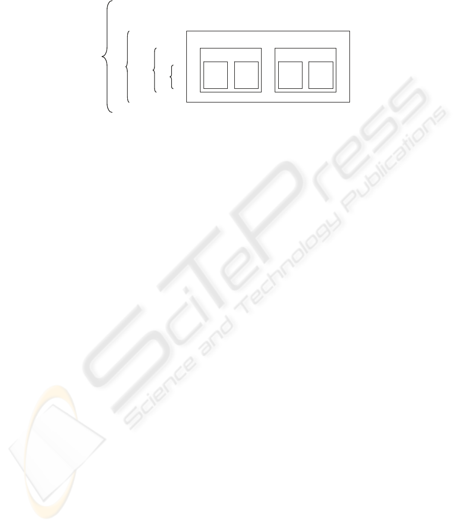
i was found to be fake, then the fakeness probability of item j increases more than that
of item k, which in turn increases more than that of item m.
Fig. 1. An illustrative item hierarchy.
We name the levels of the hierarchy as shown in Fig. 1:
• l
1:
The deepest level of the hierarchy where objects in an aggregation are uniquely
identifiable, e.g.
Items being together in the same case.
• l
2:
The next level of the hierarchy, e.g.
cases being together on the same palette.
• l
3:
The next level of the hierarchy, e.g.
palettes being together in the same container.
• l
n
: The last level of the hierarchy.
As we indicated earlier, the hierarchy structures support different concepts of
proximity such as the mentioned case-pallet-container proximity, but also proximity
due to supply chain partner ownership or the combination of these two. In the
simulation study of section 3, we will consider proximity due to partner ownership,
but this does not change anything in the structures or algorithms discussed in this
section.
We introduce the notation l(a,b), which denotes the deepest level of the hierarchy
containing items a & b. Thus we have from Fig. 1 that l(i,j) = l
1;
l(i,k) = l
2;
l(i,m) = l
3.
A
x
denotes an aggregation at level x, so the aggregation containing items i and j but
not k is an A
1
aggregation where as the aggregation containing all three items but not
m and n is an A
2
aggregation.
Probability Calculation Algorithms. In this section, the two algorithms for fakeness
probability calculation are discussed. The following outlined definitions are needed:
• H is a hierarchy of items at hand as shown in Fig. 1 with cardinal |H| (the number
of items in the hierarchy)
•
)(, ipHi ∈∀
is the fakeness probability of i,
[
]
1,0)(
∈
ip
• Items in H are grouped in conceptual aggregations A shown as boxes in Fig. 1
• U
A
is the set of unverified items of aggregation A with cardinal |U
A
|,
AU
A
⊂
• V
A
is the set of already verified items of aggregation A with cardinal |V
A
|,
AV
A
⊂
• |V
A
| + |U
A
| = |A|
ij k m
l
1
l
2
l
3
l
n
.
.
.
nij k m
l
1
l
2
l
3
l
n
.
.
.
n
103

• F
A
is the subset of V
A
where checked items were found to be fake, cardinal |F
A
|,
A
Fiip ∈
∀
= ,1)(
• G is the subset of C
A
where checked items were found to be genuine, cardinal |G
A
|,
A
Giip ∈
∀
= ,0)(
• |F
A
| + |G
A
| = |V
A
|
The first algorithm calculates a fakeness coefficient for yet-unchecked items in the
hierarchy based on their proximity to already-found genuine and fake items. An item
which is closer to fakes and further away from genuine items will have a high
fakeness coefficient. Adjustable parameters are used to specify the relative
importance of the different proximity levels. Finally, the fakeness coefficients are
used as weights to determine a fakeness probability for each unchecked item.
In the second algorithm, we maintain two values for each aggregation in the
hierarchy: a value P denoting the percentage of already verified items which are fake,
and a value C which is a confidence value denoting the percentage of items in the
aggregation which were already checked. The fakeness probability of each item is
then determined by considering the P and C values of all its parent aggregations,
weighted by adjustable parameters as in the first algorithm.
The algorithms are detailed below.
First Algorithm. This approach consists of two parts:
1. Determining the average fakeness probability of a yet untested item in an item
hierarchy, based on the results of the tests already made on the items in the
hierarchy
2. Using this average result to calculate the fakeness probability of each (yet untested)
item in the hierarchy based on it proximity from discovered authentic and fake
items
Determining the Average Fakeness Probability P
av..
k is a coefficient that shows the
relative importance of previous tests, i.e. the correlation they have on subsequent
tests. It is a heuristic measure which reflects the acceleration with which P
av
increases
and approaches 100% each time a new counterfeit is detected , k ≥ 1. P
av
is
consequently obtained as shown in equation 1.
||||
||
HH
H
UVk
Fk
Pav
+
=
(1)
Proximity Coefficients.We use heuristic coefficients to formalize the concept of
spatial proximity, namely the relationship between finding a fake/authentic item and
the chances of finding other fake/authentic items at different levels of the hierarchy.
Using the example of Fig. 1, the proximity coefficients specify the increase in p(j)
relative to that of p(k) and p(m) upon finding that item i is counterfeit. We use the
following notation to formalize the proximity coefficients:
• PC
f
(l
x
)= PC
f
(x) is the proximity coefficient for having a fake at a level l
x
• PC
a
(l
x
)= PC
a
(x) is the proximity coefficient for having a genuine item at a level l
x
104

We will use the following shorthand:
PC
f
(l(a,b))= PC
f
(a,b) (2)
The higher the coefficients, the more significant the proximity is at the respective
level of the hierarchy, so:
)(...)2()1( nPCPCPC
fff
≥≥≥ and
)(...)2()1( nPCPCPC
aaa
≥≥≥
Algorithm to Calculate per Item Coefficients and Probabilities.
Uuuu
n
∈}...,,{
,21
are the yet-unchecked items whose fakeness probability we
want to calculate. The fakeness coefficients of these items are determined as follows:
∑
∑
∈∈
−=∈∀
Gj
a
Fj
fi
jiPFjiPFKUi ),(),(,
(3)
Given that
av
H
Ui
i
P
U
Kx
=
∑
∈
||
, we calculate x and subsequently for each unchecked item,
i
xKip =)(
.
Second Algorithm. In this algorithm, we maintain for each aggregation A two values:
P(A) and C(A):
• P(A) shows the static probability (derived from the already checked items) that an
item in A is fake:
A
A
V
F
AP =)(
(4)
• C(A) shows the confidence in the value of P(A), and it depends on the number of
checks already done as a ratio of the total number of items in A:
AA
A
UV
V
AC
+
=)(
(5)
For each authenticity check that is done on an item i, an update is made to the values
of P(A) and C(A)
AiA ∈∀
(the update propagates up the tree from i to the root
of H). After the updates to P(A) and C(A), the probability of each unverified item in
the hierarchy is calculated as the weighted mean of the probabilities of its containing
aggregations. The weights are the products of the confidence factors and proximity
coefficients.
105

1,,
)(
)()(
)(,
1
1
=∈=∈∀
∑
∑
=
=
nl
n
l
ll
n
l
lll
kAu
ACk
ACAPk
upUu
(6)
k
l
is a proximity coefficient similar to those in the first algorithm but always relative
to the nth level of the hierarchy.
3 Simulation
In order to evaluate the characteristics and appropriateness of both algorithms for
finding counterfeits in a supply chain, a simulation study was conducted that modeled
sample supply chains. Shipments between supply chain partners had normally
distributed lead times. Collections of counterfeits were inserted at random locations in
the supply chain and eventually detected by simulated routine checks that occurred
with a certain ratio (x % of all incoming items were checked for authenticity at any
read point).
In order to reduce the complexity of the simulation, checks were always successful
in differentiating between authentic and fake items, but the application of a check was
associated with a constant cost factor. Accordingly, the number of checks to be
performed in order to reach a certain level of confidence in a supply chain’s integrity
is an optimization goal for any product authentication strategy, so that the main target
measure of the simulation were the resources necessary to detect a similar amount of
counterfeits for the different authentication algorithms.
After the first counterfeit was detected, the number of checks in the supply chain
increased by a certain response factor in order to reflect the countermeasures that
would occur in reality after the detection of counterfeited products. This response
factor is a key characteristic of the response biases in different industries, as e.g. the
potential damage of the brand value for fake luxury goods such as high end watches
would definitely lead to a higher increase of the response factor than the detection of
non-branded low profile goods as e.g. the recently discovered flood of fake storage
media [5]. We distributed the remaining checks (after the first counterfeit was
detected) over all locations, so that the overall costs remain equal, but the number of
checks per location may differ according to the items probabilities.
We tested three scenarios in each simulation run, namely the two competing
algorithms and a baseline case. No knowledge about supply chain proximity was
utilized in the baseline case, so the items checked after the first incident were selected
randomly. For the two scenarios relying on supply chain proximity algorithms, the
items after the first incident were constantly ranked by their respective fakeness
probabilities and checked in that order. This reflected the central approach of both
algorithms, i.e. that items in close proximity to known fakes have a higher probability
of also being fake.
106
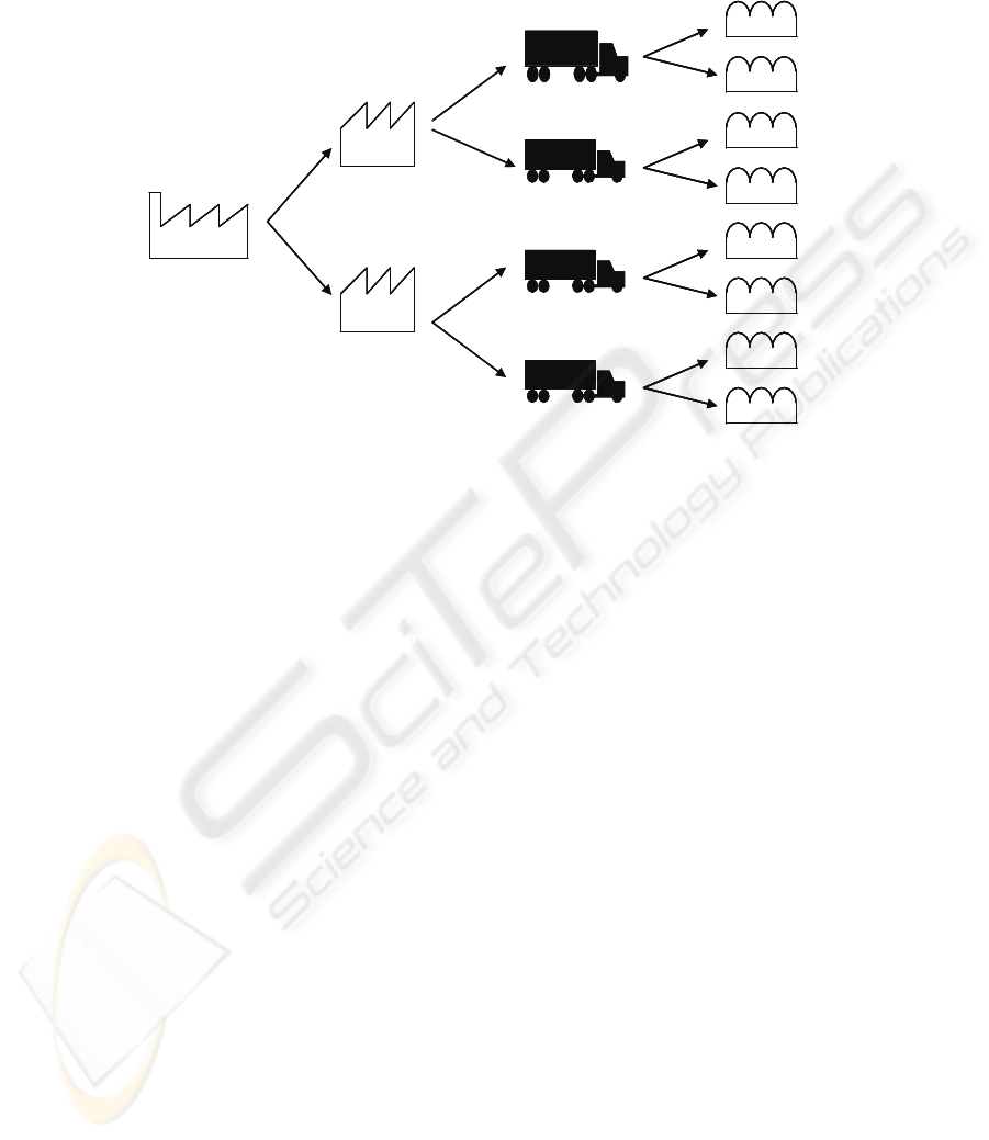
Fig. 2. The sample supply chain used for the reference simulation.
3.1 Base Case Simulation
We first conducted a base case simulation that was taken as a reference for the
respective sensitivity analysis. The base case consisted of 3000 runs of a simulation of
2000 items shipped in a supply chain with four levels of partners, organized as in a
binary tree as shown in Fig. 2. The lead time for any shipment between two partners
was normally distributed with a mean of two days and a standard deviation of half a
day. The probability that fakes were injected at any partner in the supply chain is 5%,
except at the manufacturer where it is 0%. In any run where fakes were injected, they
constituted 10% of the shipment of the owning partner. In the absence of counterfeits,
each partner randomly checked 5 items and shipped his container to the next two
partners. The total number of checks was doubled in the case of a detected counterfeit
and checks were coordinated between all locations. The coefficient k of the first
algorithm had a value of 2. The proximity coefficients PC
f
(1), PC
f
(2), and PC
f
(3) had
the values 10, 2, and 0.5 respectively, which were used for both algorithms. The
proximity coefficients PC
a
(1), PC
a
(2), and PC
a
(3), needed only for the first algorithm,
had the values 0.1, 0.05, and 0.01 respectively. All the base case parameters are
summarized in
Table 1.
Manufacturer Wholesalers
Logistics
providers
Retailers
Manufacturer Wholesalers
Logistics
providers
Retailers
107

Table 1. Base case parameters.
The results of the base case simulation showed a 5.8 and 5.6-fold increase in the
number of fakes detected using the first and second algorithm respectively as opposed
to the baseline case where no algorithm was used. A ratio which is a particularly
important measure for each algorithm is that of the fakes detected over the total
number of checks performed when fakes where actually injected. The baseline case
had a fakes/checks ratio of 2.8%, where as the cases using the first and second
algorithms had ratios of 16.5% and 15.9% respectively. The results are summarized in
Table 2.
Table 2. Results of the base case simulation.
3.2 Sensitivity Analysis
We present in this section a sensitivity analysis of the simulation where we varied one
parameter in
Table 1 at a time while keeping the others constant. We doubled and
halved each considered parameter to study its influence on the results of the base case.
Total Number of Items. The first parameter we varied was the size of the shipments
flowing in our supply chain which was 2000 items in the base case. The first
algorithm didn’t show a significant difference in results when we varied this
parameter, where as the second algorithm performed worse than the first with 1000
items and slightly better with 4000 items Table 3 summarizes the results.
Parameter Value
Total number of items 2000
Mean lead time (days) 2
Standard deviation lead time (Days) 0.5
Fake injection probability at manufacturer 0%
Fake injection probability at wholesalers 5%
Fake injection probability at logistics providers 5%
Fake injection probability at retailers 5%
Percentage of genuines replaced when fakes are injected 10%
Number of checks per partner before first fake detected 5
Factor increase in total checks when first fake detected 2
k 2
PCf(1), PCf(2), PCf(3) 10, 2, 0.5
PCa(1), PCa(2), PCa(3) 0.1, 0.05, 0.01
Case Increase in fakes detected Fakes/Checks
Without probabilities 1 2.8%
First algorithm 5.8 16.5%
Second algorithm 5.6 15.9%
108

Table 3. Results from varying the total number of items.
Standard Deviation of Lead Times. The next parameter that we vary is the standard
deviation of the normally distributed shipment time, which was 0.5 days in the base
case. We halved this value and then doubled it to examine the effect on the simulation
results. Both algorithms performed slightly worse than the base case when the
standard deviation decreased. This is an expected outcome since when different
downstream partners receive shipments without a significant delay, there will be less
chance for performed checks at one partner to influence those at the other. The results
are shown in Table 4.
Table 4. Results from varying the standard deviation of the lead times.
Fake Injection Probability at Different Locations. To study the effect of the supply
chain location where fakes were injected, we varied the probability that fakes are
injected at wholesalers, logistics providers, and retailers. For each we doubled the
initial probability of 5% to 10% keeping all other variables constant and compared the
results. The simulation demonstrates, according to the numbers in Table 5, that the
earlier in the supply chain the injection of fakes occurs, the better the results of all
cases. This is expected since the earlier the fakes are injected, the higher is the chance
to detect them at a subsequent partner. For example, if most fakes are injected at the
retailer stage, there will not be enough checks of counterfeit items to provide the
required proximity information. This explains why, when compared with the base
case, the numbers show worse performance of the algorithms when more fakes are
injected at the retailers, similar results when more fakes are injected at the logistics
providers, and better performance when the injections occur at the wholesalers.
Case Increase in fakes detected Fakes/Checks
1000 items
Without probabilities 1 2.8%
First algorithm 5.3 16.1%
Second algorithm 3.8 10.9%
4000 items
Without probabilities 1 2.8%
First algorithm 5.6 16.0%
Second algorithm 5.7 16.2%
Case Increase in fakes detected Fakes/Checks
0.25 days
Without probabilities 1 2.9%
First algorithm 5.6 16.1%
Second algorithm 5.4 15.5%
1 day
Without probabilities 1 2.7%
First algorithm 5.8 15.5%
Second algorithm 5.5 14.9%
109

Table 5. Results from varying the fake injection probability at different partners.
Percentage of Replaced Genuine Items. The next parameter we studied was the
percentage of genuine items of the respective partner’s shipment which is replaced by
counterfeits each time there was a successful injection of fakes. The base case value
of 10% was halved and doubled and resulted in the numbers shown in Table 6. The
three cases show a higher number of fakes detected which is a result of the higher
number of injected fakes. Compared to the base case, both algorithms perform
slightly worse when the percentage of replaced items is doubled or halved.
Table 6. Results from varying the percentage of genuines replaced.
Factor Increase in Total Checks when the First Fake is Detected. As mentioned
earlier, when the first fake item is detected in the supply chain, the total number of
checks to be performed in the supply chain increases by a constant factor. This factor
was 2 in the base case and was halved and doubled in our sensitivity analysis to
produce the results shown in Table 7. The numbers show that even without increasing
the number of checks when a fake is found, the two algorithms detect around 4 times
more fakes than if no algorithm is used
Case Increase in fakes detected Fakes/Checks
10% at wholesalers
Without probabilities 1 3.3%
First algorithm 5.9 19.7%
Second algorithm 5.7 18.9%
10% at logistics providers
Without probabilities 1 2.8%
First algorithm 5.9 16.3%
Second algorithm 5.7 15.8%
10% at retailers
Without probabilities 1 2.6%
First algorithm 5.4 13.8%
Second algorithm 5.3 13.5%
Case Increase in fakes detected Fakes/Checks
5% replaced
Without probabilities 1 1.5%
First algorithm 5 7.4%
Second algorithm 4.9 7.3%
20% replaced
Without probabilities 1 5.7%
First algorithm 5.5 31.2%
Second algorithm 5.4 30.6%
110

Table 7. Results from varying the factor increase in the performed checks.
Coefficient k. The coefficient k is used only in the first algorithm as a heuristic
measure to express the correlation between the results of different item checks. k’s
base value of 2 was reset to 1 and 4 to see if any significant changes occur in the first
algorithm’s performance. The results, shown in Table 8, suggest that there is no
significant effect for the value of k on the performance of the simulation.
Table 8. Varying the coefficient k of the first algorithm.
Proximity Coefficients. The final parameter we studied was the set of proximity
coefficients PC
f
which were used for both algorithms. We doubled and halved each of
PC
f
(1), PC
f
(2), and PC
f
(3) at a time while keeping all others constant. The results in
each of the 6 simulations didn’t significantly differ from the base case results, thus we
omitted the respective tables.
Supply Chain Depth. A factor whose effect has to be investigated more closely is the
structure of the supply chain itself. All the simulations until now where conducted
with the supply chain shown in Fig. 2, which resembles a binary tree of depth 3. Just
for illustration, we cut one of the levels of the supply chain, reducing it’s depth to 2,
and ran the simulation with the base case parameters. The results, documented in table
9, show that different behaviors should be expected in different supply chains. In
particular, when a supply chain is shorter, there will be less chances that enough
checks are made to obtain accurate fakeness probability value for unchecked items.
Case Increase in fakes detected Fakes/Checks
Factor increase = 1
Without probabilities 1 2.7%
First algorithm 4.1 11.3%
Second algorithm 4.1 11.2%
Factor increase = 4
Without probabilities 1 2.9%
First algorithm 6.1 17.6%
Second algorithm 5.7 16.4%
Case Increase in fakes detected Fakes/Checks
k = 1
Without probabilities 1 2.9%
First algorithm 5.6 16.2%
Second algorithm 5.4 15.9%
k = 4
Without probabilities 1 2.8%
First algorithm 5.8 16.1%
Second algorithm 5.6 15.7%
111

Table 9. Results from a depth 2 supply chain.
3.3 Discussion
As the results from the simulation indicate, both algorithms perform significantly
(more than five times) better than the baseline condition. Likewise, as the sensitivity
analysis regarding the various parameters suggests, both algorithms are relatively
robust against variations of key parameters and outperform the base condition in any
case. Hence, it is definitely worthwhile to further explore the applicability and
preconditions of both algorithms beyond the initial simple simulation study that we
have presented in this paper.
From the current insights gained from the simulation it appears that the second
algorithm is more susceptible for variations in the overall item count, resulting in
relatively weaker performance for smaller amounts of items. We will explore this
observation in the future. For now, this is the only significant difference in
performance we could find for both algorithms. Since the sensitivity analysis also
revealed a negation of this effect for an increased item count (where the second
algorithm even performed slightly better than the first), we might encounter different
applicabilities of both algorithms for different magnitudes of items in a supply chain.
The sensitivity analysis contributes also to a validation of the simulation itself, as
the variation of certain parameters such as the number of performed checks or the
lead time resulted in consistent measures exactly as one would predict from common
knowledge.
4 Related Work
We draw our assumption that the approach of supply chain proximity will be feasible
due to the supply chain partners being willing to share information from a study by
[6]. The authors analyze the impact of various levels of supply chain information
sharing including order, inventory, and demand information, which is based on
transaction costs. The study further examines the effects on supply chain performance
with a multi-agent simulation system. The findings indicate that the more detailed
information shared between firms, the lower the total cost, the higher the order
fulfillment rate, and the shorter the order cycle time. Since supply chains with high
information sharing and collaboration have a positive effect on vital business goals,
we believe that this sharing of information will also be synergistically used for the
exchange of product authentication information.
Since security and privacy issues are crucial for supply chain information exchange
and therefore also for the approach discussed in this paper, it is important to ensure
secure data access in order to realize implementations based on our proposed
Case Increase in fakes detected Fakes/Checks
Without probabilities 1 3.6%
First algorithm 2.9 10.5%
Second algorithm 2.8 10.2%
112

approach. Accordingly, [7] discuss current solutions to RFID security and privacy in
supply chains. The authors propose a security concept which exploits randomized
read access control and thus prevents hostile tracking and man-in-the-middle attacks
that is also suitable for RFID systems with a large number of tags. For future pilot
implementations of our approach we will consider similar security mechanisms.
Our core assumption is that knowing the previous and possibly the current location
of items in the supply chain can help determine their authenticity [8]. This is also
exploited in [9] which explores location-based product authentication in a situation
where only the past locations of products that flow in a supply chain are known. The
solution presented there transforms location-based authentication into a pattern
recognition problem and investigates different solutions based on machine-learning
techniques. The proposed solutions are also studied with computer simulations that
model the flow of genuine and counterfeit products in a generic pharmaceutical
supply chain. The results suggest that machine-learning techniques could be used to
automatically identify suspicious products from the incomplete location information.
However, the level of security of the studied methods, in terms of probability to detect
the clones, is relatively low, nevertheless we draw from the method of conducting a
respective simulation study from their work.
5 Outlook
What we have presented so far is a new approach for detecting counterfeits in an
RFID enabled supply chain using proximity information of items that can be gathered
by EPCIS or similar services. We have presented appropriate data structures and two
different algorithms that implement the concept of proximity based authentication.
We have illustrated the concept with a simple supply chain simulation that
demonstrated the potential benefits of our approach.
At the current point in time, our work is preliminary, since we have made quite a
few assumptions that we still have to prove. For instance, we let the number of checks
in the supply chain increase by a certain response factor that should reflect
countermeasures. We must now validate and check in how far this is really the case in
real anti counterfeiting activities, and most importantly, we must access how such a
response factor would typically differ in various industries. Correspondingly, many of
the simulation parameters presented in
Table 1 are not yet based on real industry
experiences, mostly because of the apparent difficulties to obtain real world data.
The most fundamental assumption we made, however, is that counterfeits really
enter the supply chain in close proximity to each other. Although it makes sense to
expect this to be the case, we cannot currently prove it. We do expect the emergence
of RFID enabled supply chains to provide better transparency and tracing of goods in
the mid term, so that potentially more data will become available on the inclusion
patterns of counterfeits for different supply chains.
In the short term, we will prototypically apply and refine our algorithms and other
anti counterfeiting applications in the context of the EU funded research project SToP
113

(Stop Tampering of Products
3
) out of the cluster of European RFID research projects
4
in which we work together with different end users from relevant industries (aviation,
pharma, aerospace) to gain insights to the specifics of the various industries and
further explore the concept of proximity based authentication. Consequently, we will
be able to expand our investigations to multiple supply chains from the respective
industries and thus perform appropriate external validations to our approach.
Acknowledgements
This work was supported by the European research project SToP (SToP Tampering of
Products, 034144).
References
1. http://www.iacc.org/media/statistics.php
2. T. Van Le, M. Burmester, M., B. de Medeiros: Universally composable and forward-secure
RFID authentication and authenticated key exchange. In Proceedings of the 2nd ACM
Symposium on information, Computer and Communications Security (Singapore, March 20
- 22, 2007).
3. J. Dittmann, L. Croce Ferri, C. Vielhauer: Hologram Watermarks for Document
Authentications, International Conference on Information Technology: Coding and
Computing (ITCC '01), 2001
4. D.L. Brock. The electronic product code (EPC): A naming scheme for objects. Technical
Report MIT-AUTOID-WH-002, MIT Auto ID Center, 2001. Available from
http://www.autoidcenter.org.
5. G. Schnurer. Schreiblähmung : Gefälschte SD-Karten auf dem Markt. c't 6/07, page 62
6. F. Lin, S. Huang, S. Lin: Effects of information sharing on supply chain performance in
electronic commerce", IEEE Transactions on Engineering Management, Vol. 49 No.3,
pp.258-68, 2002
7. G. Xingxin, A. Xiang, H. Wang, J. Shen, J. Huang, S. Song: An Approach to Security and
Privacy of RFID System for Supply Chain," cec-east, pp. 164-168, IEEE International
Conference on E-Commerce Technology for Dynamic E-Business (CEC-East'04), 2004
8. T. Staake, F. Thiesse, E. Fleisch: Extending the EPC Network – The Potential of RFID in
Anti-Counterfeiting. In Proceedings of the 2005 ACM symposium on Applied computing.
2005.
9. M. Lehtonen, F. Michahelles, E. Fleisch: Probabilistic Approach for Location-Based
Authentication. In The First International Workshop on Security for Spontaneous
Interaction, UbiComp. 2007
3
www.stop-project.eu
4
www.rfid-in-action.eu/cerp
114
