
ON THE PERFORMANCE OF FAULT SCREENERS IN SOFTWARE
DEVELOPMENT AND DEPLOYMENT
∗
Rui Abreu, Alberto Gonz´alez, Peter Zoeteweij and Arjan J. C. van Gemund
Software Technology Department, Faculty of Electrical Engineering, Mathematics, and Computer Science
Delft University of Technology, P.O. Box 5031, NL-2600 GA Delft, The Netherlands
Keywords: Error detection, program invariants, analytic model, fault localization, program spectra.
Abstract: Fault screeners are simple software (or hardware) constructs that detect variable value errors based on unary
invariant checking. In this paper we evaluate and compare the performance of two low-cost screeners (Bloom
filter, and range screener) that can be automatically integrated within a program, while being automatically
trained during the testing phase. While the Bloom filter has the capacity of retaining virtually all variable
values associated with proper program execution, this property comes with a much higher false positive rate
per unit training effort, compared to the more simple range screener, that compresses all value information in
terms of a single lower and upper bound. We present a novel analytic model that predicts the false positive
and false negative rate for both type of screeners. We show that the model agrees with our empirical findings.
Furthermore, we describe the application of both screeners, where the screener output is used as input to a
fault localization process that provides automatic feedback on the location of residual program defects during
deployment in the field.
1 INTRODUCTION
In many domains such as consumer products the
residual defect rate of software is considerable, due to
the trade-off between reliability on the one hand and
development cost and time-to-market on the other.
Proper error detection is a critical factor in success-
fully recognizing, and coping with (recovering from)
failures during the deployment phase (Patterson et al.,
2002; Kephart and Chess, 2003). Even more than
during testing at the development phase, errors may
otherwise go unnoticed, possibly resulting in catas-
trophic failure later.
Error detection is typically implemented through
tests (invariants) that usually trigger some excep-
tion handling process. The invariants range from
application-specific (e.g., a user-programmed test to
assert that two state variables in two different com-
ponents are in sync) to generic (e.g., a compiler-
generated value range check). While application-
specific invariants cover many failures anticipated by
the programmer and have a low false positive and
∗
This work has been carried out as part of the TRADER
project under the responsibility of the Embedded Systems
Institute. This project is partially supported by the Nether-
lands Ministry of Economic Affairs under the BSIK03021
program.
false negative rate
1
, their (manual) integration within
the code is typically a costly, and error-prone pro-
cess. Despite the simplicity of generic invariants,
and their higher false positive and false negative rate,
they can be automatically generated within the code,
while their application-specific training can also be
automatically performed as integral part of the test-
ing process during the development phase. Further-
more, generic invariants correlate to some extent with
application-specific invariants. Consequently, viola-
tion of the latter is typically preluded by violation of
the former type (Ernst et al., 1999).
In view of the above, attractive properties, generic
invariants, often dubbed fault screeners, have long
been subject of study in both the software and the
hardware domain (see Section 6). Examples include
value screeners such as simple bitmask (Hangal and
Lam, 2002; Racunas et al., 2007) and range screen-
ers (Hangal and Lam, 2002; Racunas et al., 2007),
and more sophisticated screeners such as Bloom fil-
ters (Hangal and Lam, 2002; Racunas et al., 2007).
In most work the screeners are used for automatic
fault detection (Abreu et al., 2008) and fault local-
ization (Hangal and Lam, 2002; Pytlik et al., 2003).
In all the above work, the performance of screen-
1
An error flagged when there is none is called false pos-
itive, while missing an error is called false negative.
123
Abreu R., González A., Zoeteweij P. and J. C. van Gemund A. (2008).
ON THE PERFORMANCE OF FAULT SCREENERS IN SOFTWARE DEVELOPMENT AND DEPLOYMENT.
In Proceedings of the Third International Conference on Evaluation of Novel Approaches to Software Engineering, pages 123-130
DOI: 10.5220/0001764601230130
Copyright
c
SciTePress

ers is evaluated empirically. While empirical informa-
tion is invaluable, no analytical performance models
are available that explain why certain screeners out-
perform other screeners. For example, it is known
that, compared to a (sophisticated) Bloom filter, a
simple range screener takes less effort to train, but
has worse detection performance (higher false neg-
ative rate). Up to now there has been no modeling
effort that supports these empirical findings.
In this paper we analytically and empirically in-
vestigate the performance of screeners. In particular,
we make the following contributions:
• We develop a simple, approximate, analytical per-
formance model that predicts the false positive
and false negative rate in terms of the variable do-
main size and training effort. We derive a model
for screeners that store each individual value dur-
ing training, and another model for range screen-
ers that compress all training information in terms
of a single range interval.
• We evaluate the performanceof both Bloom filters
and range screeners based on instrumenting them
within the Siemens benchmark suite, which com-
prises a large set of program versions, of which a
subset is seeded with faults. We show that our em-
pirical findings are in agreement with our model.
• As a typical application of screeners, we show
how the Bloom filter and range screeners are ap-
plied as input for automatic fault localization,
namely spectrum-based fault localization (SFL).
It is shown that the resulting fault localization ac-
curacy is comparable to one that is traditionally
achieved at the design (testing) phase.
The paper is organized as follows. In the next section
we introduce the Bloom filter and range screeners. In
Section 3 the experimental setup is described and the
empirical results are discussed. Section 4 presents
our analytical performance model. The application of
screeners as input for SFL is discussed in Section 5.
A comparison to related work appears in Section 6.
Section 7 concludes the paper.
2 FAULT SCREENERS
Program invariants, first introduced by Ernst et
al. (Ernst et al., 1999) with the purpose of support-
ing program evolution, are conditions that have to
be met by the state of the program for it to be cor-
rect. Many kinds of program invariants have been
proposed in the past (Ernst et al., 1999; Ernst et al.,
2007; Racunas et al., 2007). In this paper, we focus
on dynamic range invariants (Racunas et al., 2007),
and Bloom filter invariants (Racunas et al., 2007),
as besides being generic, they require minimal over-
head (lending themselves well for application within
resource-constrained environments, such as embed-
ded systems).
Range invariants are used to represent the (inte-
ger or real) bounds of a program variable. Every time
a new value v is observed, it is checked against the
currently valid lower bound l and upper bound u ac-
cording to
violation = ¬(l < v < u) (1)
If v is outside the bounds, an error is flagged in error
detection mode (deployment phase), while in training
mode (development phase) the range is extended ac-
cording to the assignment
l := min(l,v) (2)
u := max(l,v) (3)
Bloom filters (Bloom, 1970) are a space-efficient
probabilistic data structures used to check if an ele-
ment is a member of a set. This screener is stricter
than the range screeners, as it is basically a compact
representation of variable’s entire history.
All variables share the same Bloom filter, which
is essentially a bit array (64KB, the size of the filter
could be decreased by using a backup filter to prevent
saturation (Racunas et al., 2007)). Each 32-bit value
v
and instruction address
ia
are merged into a single
32-bit number
g
:
g = (v∗2
16
) ∨(0xFFFF ∧ia) (4)
where ∨ and ∧ are bitwise operators, respectively.
This number
g
is used as input to two hash functions
(h
1
and h
2
), which index into the Bloom filter
b
. Dur-
ing training mode, the outputs of the hash functions
are used to update the Bloom filter according to the
assignment
b[h
1
(g)] := 1; b[h
2
(g)] := 1 (5)
In detection mode an error is flagged according to
violation = ¬(b[h
1
(g)] ∧b[h
2
(g)]) (6)
3 EXPERIMENTS
In this section the experimental setup is presented,
namely the benchmark set of programs, the workflow
of the experiments, and the evaluation metrics. Fi-
nally, the experimental results are discussed.
ENASE 2008 - International Conference on Evaluation of Novel Approaches to Software Engineering
124
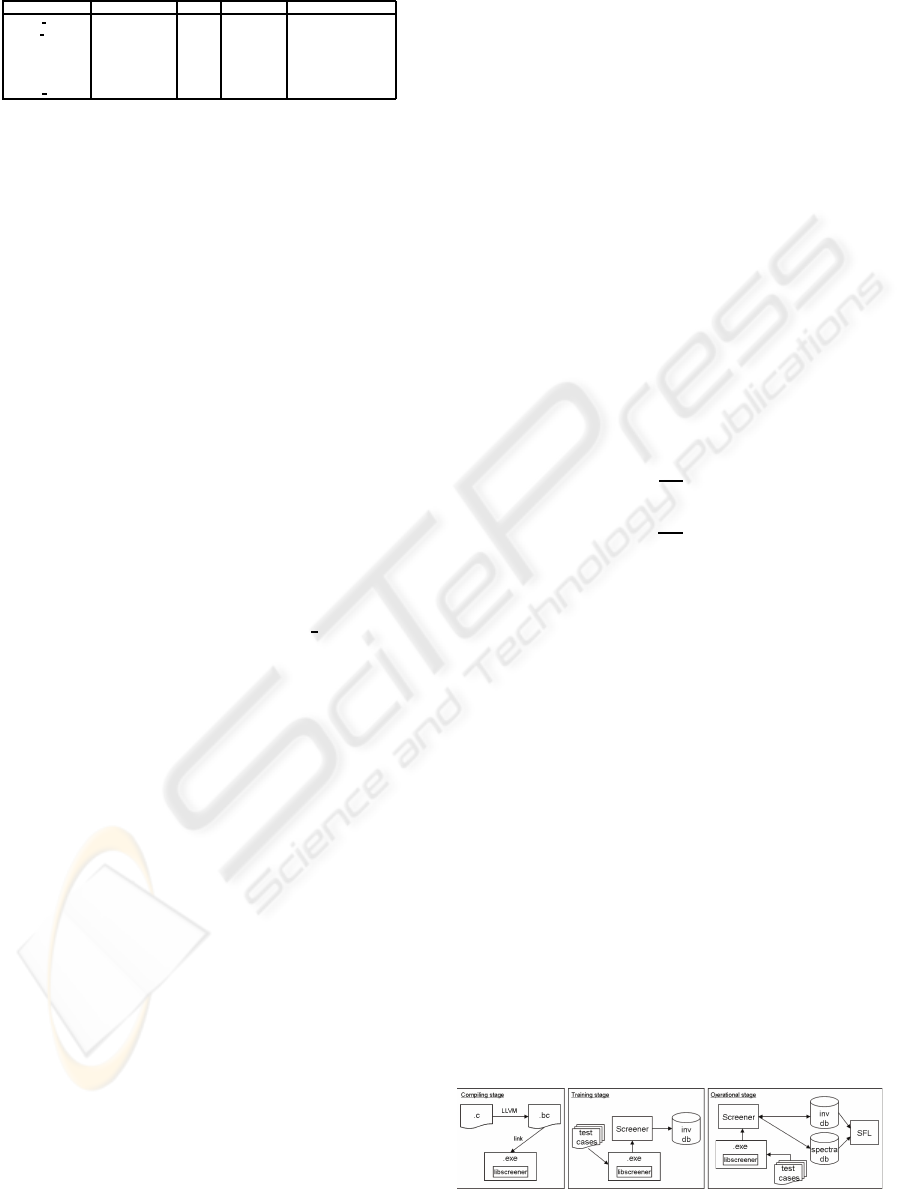
Table 1: Set of programs used in the experiments.
Program Faulty Versions LOC Test Cases Description
print tokens
7 539 4130 Lexical Analyzer
print tokens2
10 489 4115 Lexical Analyzer
replace
32 507 5542 Pattern Recognition
schedule
9 397 2650 Priority Scheduler
schedule2
10 299 2710 Priority Scheduler
tcas
41 174 1608 Altitude Separation
tot info
23 398 1052 Information Measure
3.1 Experimental Setup
Benchmark Set. In our study, we use a set of test
programs known as the Siemens set (Hutchins et al.,
1994). The Siemens set is composed of seven pro-
grams. Every single program has a correct version
and a set of faulty versions of the same program. The
correct version can be used as reference version. Each
faulty version contains exactly one fault. Each pro-
gram also has a set of inputs that ensures full code
coverage. Table 1 provides more information about
the programs in the package (for more information
see (Hutchins et al., 1994)). Although the Siemens
set was not assembled with the purpose of testing fault
diagnosis and/or error detection techniques, it is typ-
ically used by the research community as the set of
programs to test their techniques.
In total the Siemens set provides 132 programs.
However, as no failures are observed in two of these
programs, namely version 9 of
schedule2
and ver-
sion 32 of
replace
, they are discarded. Besides, we
also discard versions 4 and 6 of
print tokens
be-
cause the faults in this versions are in global variables
and the profiling tool used in our experiments does not
log the execution of these statements. In summary, we
discarded 4 versions out of 132 provided by the suite,
using 128 versions in our experiments.
Workflow of Experiments. Our approach to study
the performance of fault screeners as error detec-
tors in the deployment phase comprises three stages.
First, the target program is instrumented to gener-
ate program spectra (used by the fault localization
technique, see Section 5) and execute the invariants
(see Figure 1). To prevent faulty programs to cor-
rupt the logged information, the program invariants
and spectra themselves are located in an externalcom-
ponent (“Screener”). The instrumentation process is
implemented as an optimization pass for the LLVM
tool (Lattner and Adve, 2004) in C++ (for details on
the instrumentation process see (Gonz´alez, 2007)).
The program points screened are all memory loads/s-
tores, and function argument and return values.
Second, the program is run for those test cases for
which the program passes (its output equals that of
the reference version), in which the screeners are op-
erated in training mode. The number of (correct) test
cases used to train the screeners is of great importance
to the performance of the error detectors at the de-
ployment (detection) phase. In the experiments this
number is varied between 5% and 100% of all correct
cases (134 and 2666 cases on average, respectively)
in order to evaluate the effect of training.
Finally, we execute the program over all test cases
(excluding training set), in which the screeners are ex-
ecuted in detection mode.
Error Detection Evaluation Metrics. We evaluate
the error detection performance of the fault screeners
by comparing their output to the pass/fail outcome per
program over the entire benchmark set. The (“cor-
rect”) pass/fail information is obtained by comparing
the output of the faulty program with the reference
program.
Let N
P
and N
F
be the size of the set of passed and
failed runs, respectively, and let F
p
and F
n
be the num-
ber of false positives and negatives, respectively. We
measure the false positive rate f
p
and the false nega-
tive rate f
p
according to
f
p
=
F
p
N
P
(7)
f
n
=
F
n
N
F
(8)
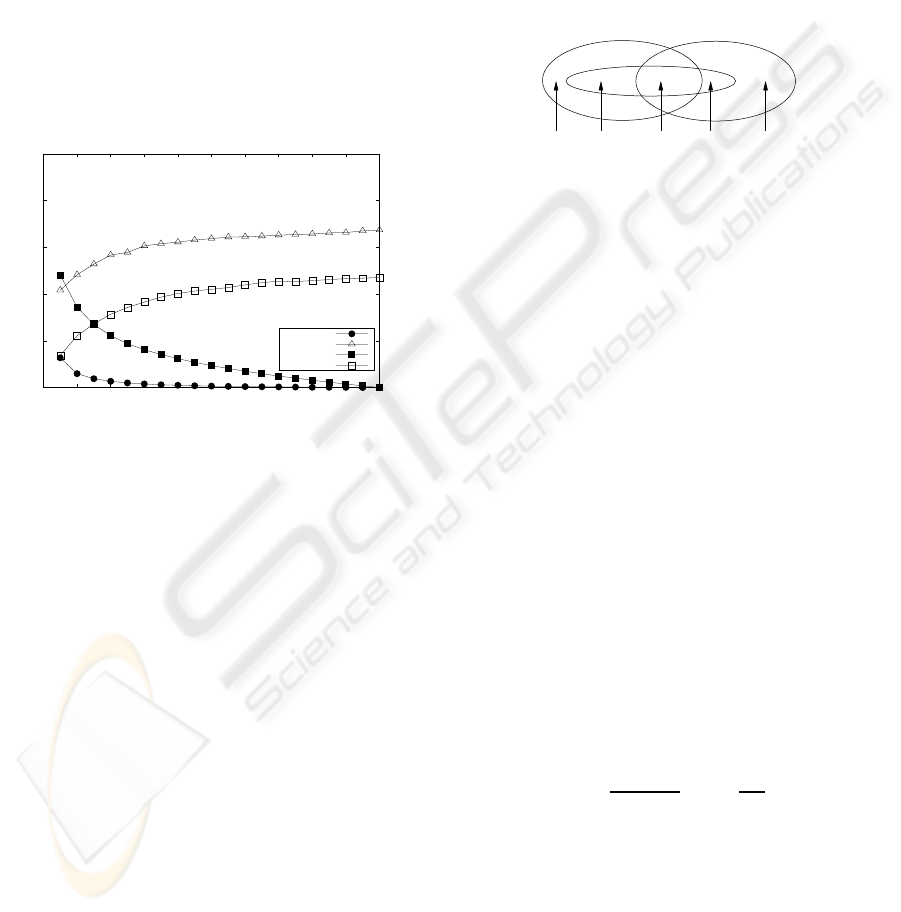
3.2 Results
Figure 2 plots f
p
and f
n
in percents for range and
Bloom filter screeners for different percentages of
(correct) test cases used to train the screeners, when
instrumenting all program points in the program un-
der analysis. The plots represent the average over
all programs, which has negligible variance (between
0 − 0.2% and 3 −5%, for f
p
and f
n
, respectively).
From the figure, the following conclusions can be
drawn for f
p
: the more test cases used to train the
screeners, the lower f
p
(as screeners evolve with the
learning process). In addition, it can be seen that
Bloom filter screeners learn slower than the range
screener. Furthermore, for both screeners f
n
rapidly
increases, meaning that even after minimal training
many errors are already tolerated. This is due to:
• limited detection capabilities: only either single
upper/lower bounds or a compact representation
of the observed values are stored are screened, i.e.,
Figure 1: Workflow of experiments.
ON THE PERFORMANCE OF FAULT SCREENERS IN SOFTWARE DEVELOPMENT AND DEPLOYMENT
125
simple and invariants, in contrast to the host of in-
variants conceivable, based on complex relation-
ships between multiple variables (typically found
in application-specific invariants)
• program-specific properties: certain variables ex-
hibit the same values for passed and failed runs,
see Section 4. Those cases lead to false negatives.
• limited training accuracy: although the plots in-
dicate that the quantity of pass/fail training input
is sufficient, the quality of the input is inherently
limited. In a number of cases a (faulty) program
error does not result in a failure (i.e., a different
output than the correct reference program). Con-
sequently, the screener is trained to accept the er-
ror, thus limiting its detection sensitivity.
0
20
40
60
80
100
0 10 20 30 40 50 60 70 80 90 100
Training %
rng fp
rng fn
bloom fp
bloom fn
Figure 2: False positives and negatives on average.
Due to its strictness, Bloom filter screeners have
on the one hand lower f
n
than range screeners. On
the other, this strictness increases f
p
. In the next sec-
tion we provide a more theoretic explanation for the
observed phenomena.
Because of their simplicity, the evaluated screen-
ers entail minimal computational overhead. On aver-
age, the 494 (203.6 variance) program points screened
introduced an overhead of 14.2% (4.7% variance) for
the range screener, and 46.2% (7.1% variance) was
measured for the Bloom filter screener (when all pro-
gram variable loads/stores and function argument/re-
turns are screened).
4 ANALYTIC MODEL
In this section we present our analytic screening per-
formance model. First, we derive some main prop-
erties that apply without considering the particular
properties that (simple) screeners exhibit. Next we
focus on the range screener, which is a typical exam-
ple of a simple screener, and which is amongst the
screeners evaluated.
4.1 Concepts and Definitions
Consider a particular program variable x. Let P de-
note the set of values x takes in all N
P
passing runs,
and let F denotes the set of values x takes in all N
F
failing runs. Let T denote the set of values recorded
during training. Let |P|,|F|,|T| denote the set sizes,
respectively. Screener performance can generally be
analyzed by considering the relationship between the
three sets P, F, and T as depicted in Fig. 3. In the fig-
P F
T
2
tn tn/fn
3 4
fp tpfn
1 5
Figure 3: Distribution of variable x.
ure we distinguish between five regions, numbered 1
through 5, all of which associate with false positives
(fp), false negatives (fn), true positives (tp), and true
negatives (tn). For example, values of x which are
within P (i.e., OK values) but which are (still) out-
side of the training set T, will trigger a false positive
(region 1). Region 3 represents the fact that certain
values of x may occur in both passing runs, as well as
failing runs, leading to potential false negatives. Re-
gion 4 relates to the fact that for many simple screen-
ers the update due to training with a certain OK value
(e.g., in region 2) may also lead to acceptance of val-
ues that are exclusively associated with failed runs,
leading to false negatives (e.g., an upper bound 10,
widened to 15 due to x = 15, while x = 13 is associ-
ated with a failed run).
4.2 Ideal Screening
In the following we derive general properties of the
evolution of the false positive rate f
p
and the false
negative rate f
n
as training progresses. For each new
value of x in a passing run the probability p that x
represents a value that is not already trained equals
p =
|P|−|T|
|P|
= 1 −
|T|
|P|
(9)
Note that for ideal screeners region 4 does not exist.
Hence T grows entirely within P. Consequently, the
expected growth of the training set is given by
t
k
−t
k−1
= p
k−1
(10)
where t
k
denotes the expected value of |T|, E[|T|], at
training step k, and p
k
denotes the probability p at step
k. It follows that t
k
is given by the recurrence relation
t
k
= α ·t
k−1
+ 1 (11)
ENASE 2008 - International Conference on Evaluation of Novel Approaches to Software Engineering
126

where α = 1−1/|P|. The solution to this recurrence
relation is given by
t
k
=
α
k
−1
α−1
(12)
Consequently
E[|T|] = |P|
1−(1−
1
|P|
)
k
(13)
Thus the fraction of T within P initially increases lin-
early with k, approaching P in the limit for k →∞.
Since in detection mode the false positive rate f
p
equals p, from (9) it follows
f
p
= (1 −
1
|P|
)
k
(14)
Thus the false positive rate decreases with k, ap-
proaching a particular threshold after a training effort
k that is (approximately) proportional to |P|. As the
false negative rate is proportional to the part of T that
intersects with F (region 3) it follows that f
n
is pro-
portional to the growth of T according to
f
n
= f
1−(1−
1
|P|
)
k
(15)
where f denotes the fraction of P that intersects with
F. Thus the false negative rate increases with k, ap-
proaching f in the limit when T equals P. From the
above it follows
f
n
= f(1− f
p
) (16)
4.3 Range Screening
In the following we introduce the constraint that the
entire value domain of variable x available for stor-
age is compressed in terms of only one range, coded
in terms of two values l (lower bound) and u (up-
per bound). Despite the potential negative impact on
f
p
and f
n
we show that the training effort required
for a particular performance is independent of the en-
tire value domain, unlike the above, general (“ideal”)
case.
After training with k values, the range screener
bounds have evolved to
l
k
= min
i=1,...,k
x
i
(17)
u
k
= max
i=1,...,k
x
i
(18)
Since x
i
are samples of x, it follows that l
k
and u
k
are essentially the lowest and highest order statis-
tic (David, 1970), respectively, of the sequence of k
variates taken from the (pseudo) random variable x
with a particular probability density function (pdf).
The order statistics interpretation allows a straight-
forward performance analysis when the pdf of x is
known. In the following we treat two cases.
4.3.1 Uniform Distribution
Without loss of generality, let x be distributed accord-
ing to a uniform pdf between 0 and r (e.g., a uniformly
distributed index variable with some upper bound r).
From, e.g., (David, 1970) it follows that the expected
values of l
k
and u
k
are given by
E[l
k
] =
1
k+ 1
r (19)
E[u
k
] =
k
k+ 1
r (20)
Consequently,
E[|T|] = E[u
k
] −E[l
k
] =
k−1
k+ 1
r (21)
Since |P| = r, from (9) it follows (f
p
= p) that
f
p
= 1 −
k−1
k+ 1
=
2
k+ 1
(22)
The analysis of f
n
is similar to the previous section,
with the modification that for simple screeners such
as the range screener the fraction f
′
of T that inter-
sects with F is generally greater than the fraction f
for ideal screeners (regions 3 and 4, as explained ear-
lier). Thus,
f
n
= f
′
(1− f
p
) = f
′
k−1
k+ 1
> f
k−1
k+ 1
(23)
4.3.2 Normal Distribution
Without loss of generality, let x be distributed accord-
ing to a normal pdf with zero mean and variance σ
(many variables such as loop bounds are measured to
have a near-normal distribution over a series of runs
with different input sets (Gautama and van Gemund,
2006)). From, e.g., (Gumbel, 1962) it follows that the
expected values of l
k
and u
k
are given by the approxi-
mation (asymptotically correct for large k)
E[l
k
] = σ
p
2log(0.4k) (24)
E[u
k
] = −σ
p
2log(0.4k) (25)
Consequently,
E[|T|] = E[u
k
] −E[l
k
] = 2σ
p
2log(0.4k) (26)
The false positive rate equals the fraction of the nor-
mal distribution (P) not covered by T. In terms of
the normal distribution’s cumulative density function
(cdf) it follows
f
p
= 1 −erf
σ
p
2log(0.4k)
σ
√
2
(27)
which reduces to
f
p
= 1 −erf
p
log(0.4k) (28)
ON THE PERFORMANCE OF FAULT SCREENERS IN SOFTWARE DEVELOPMENT AND DEPLOYMENT
127
Note that, again, f
p
is independent of the variance of
the distribution of x. For the false negative rate it fol-
lows
f
n
= f
′
(1− f
p
) = f
′
erf
p
log(0.4k) (29)
4.4 Discussion
Both the result for uniform and normal distributions
show that the use of range screeners implies that the
false positive rate (and, similarly, the false negative
rate) can be optimized independent of the size of the
value domain. Since the value domain of x can be
very large this means that range screeners require
much less training than “ideal” screeners to attain
bounds that are close to the bounds of P. Rather than
increasing one value at a time by “ideal” screeners,
range screeners can “jump” to a much greater range at
a single training instance. The associated order statis-
tics show that |T| approaches |P| regardless their ab-
solute size. For limited domains such as in the case of
the uniform pdf the bounds grow very quickly. In the
case of the normal pdf the bounds grow less quickly.
Nevertheless, according to the model a 1 percent false
positive rate can be attained for only a few thousand
training runs (few hundred in the uniform case).
The model is in good agreement with our empiri-
cal findings (see Figure 2). While exhibiting better f
n
performance, the Bloom filter suffers from a less steep
learning curve ( f
p
) compared to the range screener.
Although it might seem that even the Bloom filter has
acceptable performance near the 100 percent mark,
this is due to an artifact of the measurement setup. For
100 percent training there are no passing runs avail-
able for the evaluation(detection) phase, meaning that
there will never be a (correct) value presented to the
screener that it has not already been seen during train-
ing. Consequently, for the 100 percent mark f
p
is zero
by definition, which implies that in reality the Bloom
filter is expected to exhibit still a non-zero false pos-
itive rate after 2666 test cases (in agreement with the
model). In contrast, for the range screener it is clearly
seen that even for 1066 tests f
p
is already virtually
zero (again, in agreement with the model).
5 FAULT SCREENERS AND SFL
In this section we evaluate the performance of the
studied fault screeners as error detector input for
automatic fault localization tools. Although many
fault localization tools exist (Cleve and Zeller, 2005;
Dallmeier et al., 2005; Jones and Harrold, 2005; Liu
et al., 2006; Renieris and Reiss, 2003; Zhang et al.,
2005), in this paper we use spectrum-based fault lo-
calization (SFL) because it is known to be among the
best techniques (Jones and Harrold, 2005; Liu et al.,
2006).
In SFL, program runs are captured in terms of a
spectrum. A program spectrum (Harrold et al., 1998)
can be seen as a projection of the execution trace that
shows which parts (e.g., blocks, statements, or even
paths) of the program were active during its execu-
tion (a so-called “hit spectrum”). In this paper we
consider a program part to be a statement. Diagno-
sis consists in identifying the part whose activation
pattern resembles the occurrences of errors in differ-
ent executions. This degree of similarity is calculated
using similarity coefficients taken from data cluster-
ing techniques (Jain and Dubes, 1988). Amongst the
best similarity coefficients for SFL is the Ochiai coef-
ficient (Abreu et al., 2007; Abreu et al., 2008; Abreu
et al., 2006). The output of SFL is a ranked list of
parts (statements) in order of likelihood to be at fault.
Given that the output of SFL is a ranked list of
statements in order of likelihood to be at fault, we de-
fine quality of the diagnosis q
d
as 1 −(p/(N −1)),
where p is the position of the faulty statement in the
ranking, and N the total number of statements, i.e.,
the number of statements that need not be inspected
when following the ranking in searching for the fault.
If there are more statements with the same coefficient,
p is then the average ranking position for all of them
(see (Abreu et al., 2008) for a more elaborate defini-
tion).
0%
20%
40%
60%
80%
100%
10% 20% 30% 40% 50% 60% 70% 80% 90% 100%
Diagnostic quality q
d
Training %
rng-Ochiai
bloom-Ochiai
Figure 4: Diagnostic quality q
d
on average.
Figure 4 plots q
d
for SFL using either of both
screeners versus the training percentage as used in
Figure 2. In general, the performance is similar.
The higher f
n
of the range screener is compen-
sated by its lower f
p
, compared to the Bloom filter
screener. The best q
d
, 81% for the range screener
is obtained for 50% training, whereas the Bloom fil-
ter screener has its best 85% performance for 100%.
From this, we can conclude that, despite its slower
learning curve, the Bloom filter screener can outper-
form the range screener if massive amounts of data
ENASE 2008 - International Conference on Evaluation of Novel Approaches to Software Engineering
128

Figure 5: Screener-SFL vs. reference-based SFL.
are available for training ( f
p
becomes acceptable).
On the other hand, for those situations where only
a few test cases are available, it is better to use the
range screener. Comparing the screener-SFL perfor-
mance with SFL at development-time (84% on aver-
age (Abreu et al., 2006), see Figure 5), we conclude
that the use of screeners in an operational (deploy-
ment) context yields comparable diagnostic accuracy
to using pass/fail information available in the testing
phase. As shown in (Abreu et al., 2008) this is due
to the fact that the quantity of error information com-
pensates the limited quality.
Due to their small overhead ((Abreu et al., 2008;
Abreu et al., 2007), see also Section 3.2), fault screen-
ers and SFL are attractive for being used as error de-
tectors and fault localization, respectively.
6 RELATED WORK
Dynamic program invariants have been subject of
study by many researchers for different purposes,
such as program evolution (Ernst et al., 1999; Ernst
et al., 2007; Yang and Evans, 2004), fault de-
tection (Racunas et al., 2007), and fault localiza-
tion (Hangal and Lam, 2002; Pytlik et al., 2003).
More recently, they have been used as error detec-
tion input for fault localization techniques, namely
SFL (Abreu et al., 2008).
Daikon (Ernst et al., 2007) is a dynamic and auto-
matic invariant detector tool for several programming
languages, and built with the intention of supporting
program evolution, by helping programmers to under-
stand the code. It stores program invariantsfor several
program points, such as call parameters, return val-
ues, and for relationships between variables. Exam-
ples of stored invariants are constant, non-zero, range,
relationships, containment, and ordering. Besides, it
can be extended with user-specified invariants. Car-
rot (Pytlik et al., 2003) is a lightweight version of
Daikon, that uses a smaller set of invariants (equal-
ity, sum, and order). Carrot tries to use program in-
variants to pinpoint the faulty locations directly. Sim-
ilarly to our experiments, the Siemens set is also used
to test Carrot. Due to the negative results reported, it
has been hypothesized that program invariants alone
may not be suitable for debugging. DIDUCE (Hangal
and Lam, 2002) uses dynamic bitmask invariants for
pinpointing software bugs in Java programs. Essen-
tially, it stores program invariants for the same pro-
gram points as in this paper. It was tested on four real
world applications yielding “useful” results. How-
ever, the error detected in the experiments was caused
by a variable whose value was constant throughout
the training mode and that changed in the deploy-
ment phase (hence, easy to detect using the bitmask
screener). In (Racunas et al., 2007) several screen-
ers are evaluated to detect hardware faults. Evaluated
screeners include dynamic ranges, bitmasks, TLB
misses, and Bloom filters. The authors concluded that
bitmask screeners perform slightly better than range
and Bloom filter screeners. However, the (hardware)
errors used to test the screeners constitute random bit
errors which, although ideal for bitmask screeners,
hardly occur in program variables. IODINE (Hangal
et al., 2005) is a framework for extracting dynamic in-
variants for hardware designs. In has been shown that
dynamic invariant detection can infer relevant and ac-
curate properties, such as request-acknowledge pairs
and mutual exclusion between signals.
To the best of our knowledge, none of the previous
work has analytically modeled the performance of the
screeners.
7 CONCLUSIONS & FUTURE
WORK
In this paper we have analytically and empirically in-
vestigated the performance of low-cost, generic pro-
gram invariants (also known as “screeners”), namely
range and Bloom-filter invariants, in their capacity
of error detectors. Empirical results show that near-
“ideal” screeners, of which the Bloom filter screener
is an example, are slower learners than range invari-
ants, but have less false negatives. As major contri-
bution, we present a novel, approximate, analytical
model to explain the fault screener performance. The
model shows that the training effort required by near-
“ideal” screeners, such as Bloom filters, scales with
the variable domain size, whereas simple screeners,
such as range screeners, only require constant train-
ing effort. Despite its simplicity, the model is in to-
tal agreement with the empirical findings. Finally,
we evaluated the impact of using such error detec-
tors within an SFL approach aimed at the deploy-
ment (operational) phase, rather than just the devel-
opment phase. We verified that, despite the simplicity
ON THE PERFORMANCE OF FAULT SCREENERS IN SOFTWARE DEVELOPMENT AND DEPLOYMENT
129

of the screeners (and therefore considerable rates of
false positives and/or negatives), the diagnostic per-
formance of SFL is similar to the development-time
situation. This implies that fault diagnosis with an ac-
curacy comparable to that in the development phase
can be attained at the deployment phase with no addi-
tional programming effort or human intervention.
Future work includes the following. Al-
though other screeners are more time-consuming and
program-specific, such as relationships between vari-
ables, they may lead to better diagnostic performance,
and are therefore worth investigating. Furthermore,
although earlier work has shown that the current di-
agnostic metric is comparable to the more common
T-score (Jones and Harrold, 2005; Renieris and Reiss,
2003), we also plan to redo our study in terms of
the T-score, allowing a direct comparison between the
use of stand-alone screeners and the screener-SFL ap-
proach. Finally, we study ways to decrease screener
density, aimed to decrease screening overhead.
REFERENCES
Abreu, R., Gonz´alez, A., Zoeteweij, P., and van Gemund,
A. (2008). Automatic software fault localization us-
ing generic program invariants. In Proc. SAC’08, For-
taleza, Brazil. ACM Press. accepted for publication.
Abreu, R., Zoeteweij, P., and van Gemund, A. (2006). An
evaluation of similarity coefficients for software fault
localization. In Proccedings of PRDC’06.
Abreu, R., Zoeteweij, P., and van Gemund, A. (2007). On
the accuracy of spectrum-based fault localization. In
Proc. TAIC PART’07.
Bloom, B. (1970). Space/time trade-offs in hash coding
with allowable errors. Commun. ACM, 13(7):422–
426.
Cleve, H. and Zeller, A. (2005). Locating causes of program
failures. In Proc. ICSE’05, Missouri, USA.
Dallmeier, V., Lindig, C., and Zeller, A. (2005).
Lightweight defect localization for Java. In Black,
A. P., editor, Proc. ECOOP 2005, volume 3586 of
LNCS, pages 528–550. Springer-Verlag.
David, H. A. (1970). Order Statistics. John Wiley & Sons.
Ernst, M., Cockrell, J., Griswold, W., and Notkin, D.
(1999). Dynamically discovering likely program in-
variants to support program evolution. In Proc.
ICSE’99, pages 213–224.
Ernst, M., Perkins, J., Guo, P., McCamant, S., Pacheco, C.,
Tschantz, M., , and Xiao, C. (2007). The Daikon sys-
tem for dynamic detection of likely invariants. In Sci-
ence of Computer Programming.
Gautama, H. and van Gemund, A. (2006). Low-cost
static performance prediction of parallel stochastic
task compositions. IEEE Trans. Parallel Distrib. Syst.,
17(1):78–91.
Gonz´alez, A. (2007). Automatic error detection techniques
based on dynamic invariants. Master’s thesis.
Gumbel, E. (1962). Statistical theory of extreme values
(main results). In Sarhan, A. and Greenberg, B., ed-
itors, Contributions to Order Statistics, pages 56–93.
John Wiley & Sons.
Hangal, S., Chandra, N., Narayanan, S., and Chakravorty,
S. (2005). IODINE: A tool to automatically infer dy-
namic invariants for hardware designs. In DAC’05,
San Diego, California, USA.
Hangal, S. and Lam, M. (2002). Tracking down software
bugs using automatic anomaly detection. In Proc.
ICSE’02.
Harrold, M., Rothermel, G., Wu, R., and Yi, L. (1998). An
empirical investigation of program spectra. ACM SIG-
PLAN Notices, 33(7):83–90.
Hutchins, M., Foster, H., Goradia, T., and Ostrand, T.
(1994). Experiments of the effectiveness of dataflow-
and controlflow-based test adequacy criteria. In Proc.
ICSE’94, Sorrento, Italy. IEEE CS.
Jain, A. and Dubes, R. (1988). Algorithms for clustering
data. Prentice-Hall, Inc.
Jones, J. and Harrold, M. (2005). Empirical evaluation of
the tarantula automatic fault-localization technique. In
Proc. ASE’05, pages 273–282, NY, USA.
Kephart, J. and Chess, D. (2003). The vision of autonomic
computing. Computer, 36(1):41–50.
Lattner, C. and Adve, V. (2004). LLVM: A Compilation
Framework for Lifelong Program Analysis & Trans-
formation. In Proc. CGO’04, Palo Alto, California.
Liu, C., Fei, L., Yan, X., Han, J., and Midkiff, S. (2006).
Statistical debugging: A hypothesis testing-based ap-
proach. IEEE TSE, 32(10):831–848.
Patterson, D., Brown, A., Broadwell, P., Candea, G., Chen,
M., Cutler, J., Enriquez, P., Fox, A., Kiciman, E.,
Merzbacher, M., Oppenheimer, D., Sastry, N., Tet-
zlaff, W., Traupman, J., and Treuhaft, N. (2002). Re-
covery Oriented Computing (ROC): Motivation, defi-
nition, techniques, and case studies. Technical Report
UCB/CSD-02-1175, U.C. Berkeley.
Pytlik, B., Renieris, M., Krishnamurthi, S., and Reiss, S.
(2003). Automated fault localization using potential
invariants. In Proc. AADEBUG’03.
Racunas, P., Constantinides, K., Manne, S., and Mukherjee,
S. (2007). Perturbation-based fault screening. In Proc.
HPCA’2007, pages 169–180.
Renieris, M. and Reiss, S. (2003). Fault localization with
nearest neighbor queries. In Proc. ASE’03, Montreal,
Canada. IEEE CS.
Yang, J. and Evans, D. (2004). Automatically inferring
temporal properties for program evolution. In Proc.
ISSRE’04, pages 340–351, Washington, DC, USA.
IEEE CS.
Zhang, X., He, H., Gupta, N., and Gupta, R. (2005). Exper-
imental evaluation of using dynamic slices for fault
location. In Proc. AADEBUG’05, pages 33–42, Mon-
terey, California, USA. ACM Press.
ENASE 2008 - International Conference on Evaluation of Novel Approaches to Software Engineering
130
