
FAULTS ANALYSIS IN DISTRIBUTED SYSTEMS
Quantitative Estimation of Reliability and Resource Requirements
Christian Dauer Thorenfeldt Sellberg
IBM Denmark A/S. Nymoellevej 91, 2800 Kgs. Lyngby, Denmark
Michael R. Hansen, Paul Fischer
Institute of Mathematical Modelling, Technical University of Denmark
Richard Petersens Plads, DTU - Building 321, 2800 Kgs. Lyngby, Denmark
Keywords: Fault tolerance, Dependable systems, Distributed systems, Process Algebra, Pi-calculus.
Abstract: We live in a time where we become ever more dependent on distributed computing. Predictable quantitative
properties of reliability and resource requirements of these systems are of outmost importance. But today
quantitative properties of these systems can only be established after the systems are implemented and
released for test, at which point problems can be costly and time consuming to solve. We present a new
method, a process algebra and simulation tool for estimating quantitative properties of reliability and
resource requirements of a distributed system with complex behaviour hereunder complex fault-tolerance
behaviour. The simulation tool allows tailored fault injection e.g. random failure and attacks. The method is
based upon π-calculus (Milner, 1999) to which it adds a stochastic fail-able process group construct.
Performance is quantitatively estimated using reaction rates (Priami, 1995). We show how to model and
estimate quantitative properties of a CPU scavenging grid with fault-tolerance. To emphasize the
expressiveness of our language called Gπ we provide design patterns for encoding higher-order functions,
object-oriented classes, process translocation, conditional loops and conditional control flow. The design
patterns are used to implement linked lists, higher-order list functions and binary algebra. The focus of the
paper--is—on--practical--application.
1 INTRODUCTION
Failure (faults) happens. The computational
resources of distributed systems are unreliable; as
every human made thing is and they will eventually
fail either because of random failure, because of
limited longevity or because of malicious attacks. To
be reliable then dependable systems need to be
robust against these different causes of failure.
Robustness against failures can e.g. be achieved via
fault-tolerance techniques.
Analysis of reliability and resource requirements
(such as performance) is usually delayed (or not
done at all) until a distributed system is implemented
and deployed, where the analysis is based on data
collected via load and stress testing, LST, of the
deployed system via LST tools. The reason for this
delay is that reliability and resource requirements of
a system are not easily deduced in the planning and
modelling phases. We need a method which allows
quantitative estimation of reliability and quantitative
estimation of predictive statistics (mean, standard
deviation, minimum, median, maximum) of resource
requirements in space and time (e.g. memory,
network size, workload, performance) based on a
model of the system. The method should be able to
account for location failure (e.g. server crash) and
fault-tolerance (fault detection, fault confinement,
fault recovery) techniques. The method should be
able to express component based job distribution to
a computational resource. Our thesis is that π-
calculus (Milner, 1999) could be extended for this
purpose and the results presented in this paper are a
summary of the results from the master thesis
(Sellberg, 2008).
Why a new process algebra? There exists
process algebras based on π-calculus (Milner, 1999)
with location failure; examples are asynchronous π
l
,
45
Dauer Thorenfeldt Sellberg C., R. Hansen M. and Fischer P. (2008).
FAULTS ANALYSIS IN DISTRIBUTED SYSTEMS - Quantitative Estimation of Reliability and Resource Requirements.
In Proceedings of the Third International Conference on Software and Data Technologies - SE/GSDCA/MUSE, pages 45-52
DOI: 10.5220/0001881700450052
Copyright
c
SciTePress

(Amadio, 1997) and DπLoc, (Francalanza, 2006).
But these process algebras have no means for
expressing quantitative aspects of reliability and
resource requirements in time and space. One
extension of π-calculus with quantitative properties
is Stochastic π-calculus, Sπ, (Priami, 1995). Sπ can
via its stochastic reaction rate extension to π-
calculus quantify system performance but Sπ has no
notion of failure.
We have considered whether we should extend
e.g. π
l
or DπLoc with quantitative properties but
have abandoned doing this for the following reasons.
π
l
and DπLoc has fault detection logic, FD, a ping
“are you alive” construct, as a part of the syntax. FD
in π
l
and DπLoc cannot fail, unlike FD in real
systems (see Section 2), so we cannot use π
l
and
DπLoc to study fault detection. Another issue is that
π
l
and DπLoc have syntactical fault injection
constructs. We prefer for clarity reasons that a model
is defining a system’s functional specification,
which does not include fault injection logic.
Therefore we introduce a new (π-calculus based)
process algebra which is able to express “location
failure” and quantitative properties of reliability and
resource requirements in time and space. Our
process algebra, named Gπ-calculus, adds to π-
calculus a stochastic fail-able process group
construct for location failure. We adapt reaction
rates from (Priami, 1995) in the form of transition
time labels (see section 3) for quantitative estimation
of performance. Component based job distribution is
expressed via a distribution rule. The semantics of
Gπ is given in the form of a structural operational
semantics (Plotkin, 1981). The emphasis will,
however, be on practical applications.
The paper has the following outline. In Section 2,
we present a motivating example and give a flavour
of how the method quantitatively can estimate
reliability and descriptive statistics of resource
requirements in time and space of a simple CPU
scavenging grid. Technical details are left to Section
6. In Section 3, we give an informal introduction to
Gπ-calculus. In Section 4 we stress the
expressiveness of Gπ by presenting design patterns
for how to use it to implement advanced behaviour.
In Section 5, we present the simulator tool which
can estimate descriptive statistics of quantitative
properties of models. In Section 6 we introduce how
to model fault-tolerance techniques by elaborating
on the example from Section 2. The paper ends with
a conclusion.
2 A MOTIVATING EXAMPLE
Dependability on a system requires that the system
has predictable reliability and predictable
quantitative resource requirements in time,
(performance), and space, e.g. network size (here
defined as the number of concurrent computers
which simultaneously is having a job assigned),
number of job distributions (the number of
assignments of a computational problem to a new
computational resource) and workload (here defined
as the number of computations/reductions). With
predictable we understand that standard deviation is
relatively low in respect to the mean and that min
and max is relatively close to the mean. We define
reliability of a system as the probability that a
system service will answer an arbitrary request in
accordance with its system specification.
We shall consider an example, a volunteering
CPU grid, CPU-GRID, from High Performance
Computing. High Performance Computing, HPC, is
today applied in solving complex computation
intensive problems. One way to achieve HPC is via
a CPU-GRID. Examples of CPU-GRIDs are:
folding@- home, seti@home and world, community
grid which respectively have the following urls:
http://folding.stanford.edu/
http://setiathome.berkeley.edu/
http://www.worldcommunitygrid.org
A CPU-GRID is in its simplest form based on a
central computer, a grid master, which has a set of
volunteering computers, CPUs, to which it can
delegate/schedule computational problems.
Volunteering computers can usually join the grid by
downloading and installing a screensaver which will
connect the volunteering computer to the grid. When
a grid master receives a job request by a grid user it
will usually break the job request into sub-problems
which it will delegate to volunteering CPUs. When a
sub-problem is solved the volunteer CPU will return
the sub-result to the grid master. The grid master
will assemble all sub-results into one final result and
return it to the user. The owner of a volunteer CPU
can at any time chose to (temporarily or indefinitely)
disconnect his CPU from the grid. From the point of
view of the grid master then this disconnection can
be considered as the failure of the sub-problem
delegated to that CPU. To insure that the CPU-
GRID can achieve reliable computing with such
unreliable computational resources it needs a fault-
tolerance strategy for handling the failure of
volunteering CPUs.
ICSOFT 2008 - International Conference on Software and Data Technologies
46
Fault-tolerance is about fault detection, fault
isolation/error assessment and fault recovery/error
correction (Tanenbaum, 2006). Fault detection in
distributed processes is achieved by timed processes,
usually called watchdogs, triggering timed e.g. “are-
you-alive” signals to a heart-beat process located at
a component under fault surveillance, e.g. a
volunteering CPU. If a timed heart-beat is missed
then a watchdog will handle it as the failure of the
volunteering CPU. The watchdog will then trigger
fault recovery by rescheduling the failed sub-
problem. This is the fault-tolerance approach
followed in our example below. Notice that race
conditions can course a heart-beat to be missed. This
will falsely trigger fault recovery and reschedule an
already ongoing job.
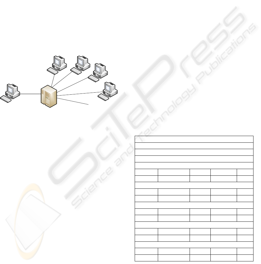
The architecture of the CPU-GRID example is
shown in Figure 1.
Figure 1: CPU-GRID architecture.
The CPU-GRID consists of a grid master and an
unlimited amount of volunteering CPUs. The user
entrance to the grid is via the grid master. The grid
master can receive a job request from a user which it
split into two sub-problems A and B which it will
schedule to volunteering CPUs. A CPU which has
been assigned a job of type A or B will be named
CpuA and CpuB resepectively. The grid master will
apply passive task replication as its fault-tolerance
strategy, i.e. it will apply watchdogs at the grid
master and heart-beat listening processes at CpuA
and CpuB for fault detection and fault recovery. The
failure probability of CpuA and CpuB is 0.5, i.e.
they are very unreliable. We consider the grid master
to have failure probability 0, i.e. it cannot fail.
We have modelled this example in Gπ and
experimented with the simulator tool. Table 1 shows
the results.
Reliability and performance are two system
properties being perceived by the grid user. The
model has high reliability but its performance is
unpredictable (standard deviation, std.dev Table 1, is
large compared to the mean) and from the point of
view of the grid user this unpredictability makes the
grid undependable.
“Network size”, “Number of job distributions”
and “System workload” are parts of the system
resources which need to be available for the CPU-
GRID for it to deliver the estimated reliability and
performance. The results show that these resource
requirements are unpredictable, but whether this
unpredictability indicates a dependability problem
depends on the actual resources available to the
CPU-GRID. If the CPU-GRID had access to e.g.
600000 volunteering computers then the resource
requirement unpredictability would probably be of
no concern but if the CPU-GRID had access to only
100 computers then it would be of concern.
The statistics for network size (Table 1) give us
an indication of the “quality” of the fault-tolerance
strategy. We can derive that fault detection wrongly
triggers fault recovery of non-failed components
because network size would be no larger than 4 (1
user, 1 grid master, 1 CpuA, 1 CpuB) if fault
detection did not fail but network size (Table 1,
Network size) is on average 7.75 and can be as large
as 16 concur rent computers.
Faults, is the number of failed volunteering
computers and can be interpreted as the “hostility”
of the environment. It seems fair to say that the
environment is relatively hostile.
Table 1: CPU scaveng. grid with passive task replication.
Total number of experiments
100.0
Reliability
1.0
Performance (times units)
mean std.dev. min median max
695,41 461,9111 49 583,5 2114
Network size
mean std.dev. min median max
7,75 2,2036 5 7 16
Number of job distributions
mean std.dev. min median max
275,72 183,368 22 229 848
System workload (reductions)
mean std.dev. min median max
2196,54 1457,3966 160 1785 6685
Faults
mean std.dev. min median max
269,52 182,1981 17 222,5 841
GridMaster
CPU
CPU
User
CPU
CPU
...
Unlimited number of
volunteering CPUs
FAULTS ANALYSIS IN DISTRIBUTED SYSTEMS - Quantitative Estimation of Reliability and Resource Requirements
47

Table 2: Structural Operational Semantics of Gπ-calculus.
Failure rules
1. […+x!y.P]
i
θi
| […+x?z.R]
j
θj
→
σi*(1-σj), ρ
0 | […+x?z.R]
j
θj
2. […+x?y.P]i
θi
| […+x!z.R]
j
θj
→
σi*(1-σj), ρ
0 | […+x!z.R ]
j
θj
3. […+x!y.P]
i
θi
| […+x?z.R]
j
θj
→
σi*σr, ρ
0 | 0
4. […+x!y.P]
i
θi
| …+x?z.R →
σi, ρ
0 | …+x?z.R
5. […+x?y.P ]
i
θi
| …+x!z.R →
σi, ρ
0 | …+x!z.R
6. […x!y.P | ...+x?z.Q]
i
θi
→
σi, ρ
0
Communication rules
1. […+x!y.P]
i
θi
| […+x?z.R]
j
θj
→
(1-σi)*(1 - σj), ρ
[P]
i
θi
| [R{y/z}]
j
θj
2. […+x!y.P ]
i
θi
| …+x?z.R →
(1-σi), ρ
[P]
i
θi
| R{y/z}
3. […+x?y.P ]
i
θi
| …+x!z.R →
(1-σi), ρ
[P{z/y}]
i
θi
| R
4. […+x!y.P | …+x?z.R]i
θi
→
(1-σi), ρ
[P | R{y/z}]
i
θi
…+x!y.P | …+x?z.R →
σ=1, ρ
P | R{z/y}
Distribution rule
[(new a1…an)(Q | [P]
θj
)]
θi
→
σ,ρ
(new a1…an)( [Q]
θi
| [P]
θj
) where σ=1 and ρ=0
3 INTRODUCTION TO
Gπ-CALCULUS
The calculus Gπ is based on the π-calculus
introduced in (Milner, 1999) for modelling and
analysing concurrent, communicating and mobile
processes. For a comprehensive introduction to π-
calculus we refer to (Milner, 1999) or (Sangiorgi,
2001). The syntax of π-calculus is shown in Table 3.
Table 3: π-calculus syntax.
P,Q ::= S | *P | (new x) P | P|Q | 0
S, T ::= α.P | S + T
α ::= a?b | a!b
See Table 4 for an explanation of terms used.
Table 4: Gπ-calculus syntax.
P,Q ::= S | *P | (new x) P | P|Q | 0 | [P]θ
S, T ::= α.P | S + T
α ::= a?b | a!b
θ ::= ε | ‘@’ name=value ‘;’ θ
Where ε is the empty string. P and Q are processes,
S and T are summations and α is an action. The
syntactic constructs have the following meaning.
π-calculus is Turing complete and therefore
allows the modelling of arbitrarily complex
behaviour, but π-calculus cannot express
quantitative properties as reliability and resource
requirements in time and space or grouped process
failure and therefore primitives to express that is
added to π-calculus.
The syntax of Gπ is given in Table 4 and the
operational semantics is sketched in Table 2.
Composition: P|Q means that P and Q are two
concurrent processes.
Prefix: α.P means sequencing of behaviour. The
process can engage in an α action and then it
behaves as P.
Action: a?b and a!b are symbolizing
communication points. a?b is an input action and a!b
is and output action. The name, a in a?b and a!b is
called the subject and b is called the object. When an
input- and output-action have the same subject-name
they can engage in communication (Table 2,
communication rules).
Summation: S + T means choice of process
behaviour where only one alternative i.e. either S or
T but nor both will evaluate, the other alternative is
discarded.
Replication: *P represents an infinite set of
process P occurrences. We have the following
structural congruence rule *P ≡ P | *P.
Restriction: (new x) P means that x is bounded in
P. In the following example (new x)(P) | (new x)(Q)
then the x’s in P and Q represents two different
names.
Termination: 0 means a terminated process, a
process that takes no action.
Grouping: [P]
θ
means process grouping. The
process group can evaluate to the null process,
[P]
θ
→0 (Table 2, failure rules). The tagging θ is a
convenient way of adding meta information to
process groupings. We use the tag @pf=0.5; for
example to indicate the failure probability of a
process group. We shall se other kinds of tags for
type in section 6.
ICSOFT 2008 - International Conference on Software and Data Technologies
48

We will now briefly explain the reason for our
failure modelling approach. The processes deployed
on a computational resource are un-reliable because
a computational resource always can fail given some
probability. The processes, so-to-speak, “inherit”
this unreliability from their computational resource,
because they cease to exist with the computational
resource. We model a computational resource by a
process group construct, [P], which we add as an
extension to the π-calculus syntax (Table 4). We
model the unreliability of the computational
resource by extending the reduction rules of π-
calculus with reduction rules of failure (Table 2).
Notice that failure is only defined for process
groups, [ ], having processes which can react; this
insures that we are only studying interesting failures
which affects behaviour.
In the operational semantics, each transition
arrow, →
σ, ρ
, has two labels. The first label, σ, is the
transition probability and the second, ρ, is the
transition time. The symbols σi and σj (Table 2) are
the probabilities that respectively the process group
marked i and j will fail during reaction. The
transition probability σi*(1-σj) is the probability for
the event that the process group marked i but not the
process group marked j will fail during reaction
(Table 2) etc. Using these transition labels we can
deduce transition path probabilities and transition
path times, to estimate reliability and performance
figures.
The semantic reduction rules for communication
trivially specify that communication will take place
when none of the involved process groups fails and
the transition probabilities are reflecting this. Job
distribution or assignment to computational
resources is specified by the distribution.
Different aspects of process size are used to
estimate resource requirements in e.g. memory and
network size. The number of times the different
reduction rules are applied is used to estimate
different aspects of work load, e.g. network traffic
and CPU load.
4 EXPRESSIVENESS
To make Gπ useable by a wide audience we have
presented six design patterns, Gπ-patterns (Table 5),
for how Gπ-calculus can be used to implement
complex behaviour via concepts familiar from the
functional or object oriented world.
The design patterns have been heavily inspired
by both (Milner, 1999) and (Sangiorgi, 2003). Each
design pattern has a name for reference, it defines a
problem or problem context where it is useful, it
defines a set of terms to be used as a vocabulary for
talking about the pattern and most importantly it
defines a Gπ process structure as a solution to the
problem. The intention is that these process
structures are to be used as coding templates which
can be modified to fit a concrete problem. We will,
for space reasons, not go into details about how
these high-level constructs can be expressed in Gπ.
Table 5: Gπ patterns overview
Pattern Problem context
Gπ-Function
Need for an implementation
of a function as known from
functional programming
Gπ-Conditional-
Loop
Need for conditional loop e.g.
do-while
Gπ-If-Equals-Then-
Else
Need for conditional control
flow
G-Higher-Order-
Function
Need for higher order
functions or subroutines.
Gπ-Class-Object
Need for an object oriented
approach
Gπ-Process-Group-
Handle
Need for process
translocation between process
groups
To demonstrate the usefulness of the Gπ-patterns
we have used them to implement Gπ functionality
on a representation of 7 bit binary numbers. All Gπ
implementations have been tested via the simulator
tool. We have implemented binary algebraic
functionality where e.g. the implementation of
binary addition makes use of the Gπ-Function, Gπ-
Conditional-Loop and Gπ-Conditional-Control-Flow
patterns. Our Gπ implementation of binary
multiplication makes among others use of the binary
addition implementation via the Gπ-Higher-Order-
Function pattern.
We have implemented linked list of binary
numbers, where each list node is implemented as an
instance of the Gπ-Class-Object pattern. The
implementation of the linked list implements object
functionality (methods) for traversing the list and for
updating the value of a specific node and for adding
new elements to the list. We have implemented
higher-order linked list function which can apply a
function to each element in the list.
The implemented Gπ functions can be
considered as the beginning of a reusable Gπ-API.
FAULTS ANALYSIS IN DISTRIBUTED SYSTEMS - Quantitative Estimation of Reliability and Resource Requirements
49
5 SIMULATOR TOOL
The simulator tool is written in Java. It has a
graphical user interface, GUI, and a command line
interface. The simulator has two main functions. It
has an interface for studying the behaviour of a Gπ-
model; A Gπ-model can be loaded into the simulator
and the user can study the behaviour of the model by
observing structural changes in the model by
applying one reduction rule at the time. The other
function is that it can be used to quantitatively
estimate reliability and descriptive statistics of
resource requirements in time and space of a Gπ-
model.
The simulator is an interpreter of the structural
operational semantics of Gπ. It reduces a Gπ model
one reduction rule at the time. After each reduction
step it collects and updates quantitative properties of
the Gπ model.
We call one execution of the simulator algorithm
on a Gπ-model for a simulation experiment. For
each simulation experiment we collect quantitative
properties. We can specify to the simulator (not
shown here, please assist (Sellberg, 2008)) what a
successful outcome is, so the simulator can decide
whether a simulation experiment was a success or
not (step number 07 in the simulator algorithm
below). This is used to estimate reliability. The
estimator part of the simulator tool will run a
simulation experiment a specified number of times
and collect quantitative properties and calculate
descriptive statistics. Reliability is estimated as the
fraction of successful simulation experiments.
Pseudo code for the simulator algorithm is given
below where the symbol Γ symbolizes the Gπ-model
to be executed.
simulate( Γ)
01: distribute (un-nest) all nested
process groups in Γ
02: randomly find matching process pair
in Γ which can react
03: if no match is found then stop else
continue
04: apply fault injection logic
05: if faults were injected then goto
step 01 else continue
06: apply reaction for found matching
process pair in Γ
07: test if a functional test evaluated
with success. If true then stop
else goto step 01
The fault injection logic and reaction rate logic is
delegated to interfaces which can be implemented to
fit specific failure and reaction rate scenarios. A Gπ
model is given as ASCII text to the simulator.
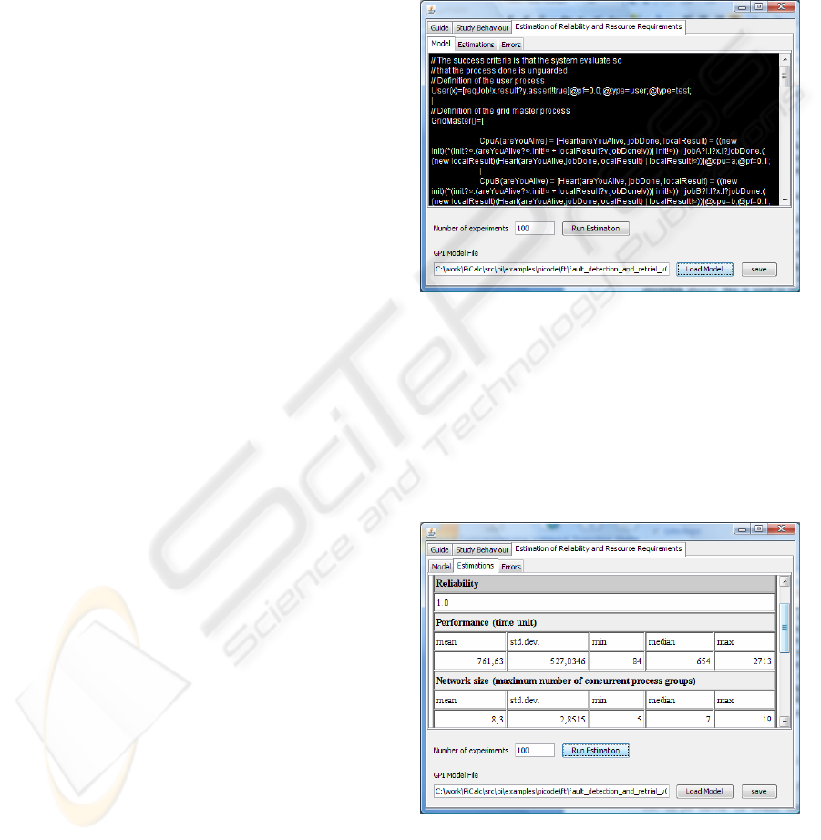
The purpose of Figure 2 and Figure 3 is to give
the reader an impression of the estimator part of the
simulators GUI.
Figure 2 shows the Gπ-model of the CPU
scavenging grid loaded from an ASCII file into the
simulator GUI. We can edit the model (and save
changes) via the black editor screen (Figure 2).
Figure 2: Gπ-model loaded into the simulator tool.
We can enter the number of simulation
experiments we want to base our estimation results
on and initiate our estimation process by pressing
the button “run estimation”. Estimation results are
presented as shown in Figure 3 and show the
estimated statistics of reliability and resource
requirements in time and space. The results have the
form presented in Table 1.
Figure 3: Result of executing a simulation.
ICSOFT 2008 - International Conference on Software and Data Technologies
50

6 FAULT-TOLERANCE
In (Sellberg, 2008) we sketch how we can use Gπ to
model relevant and interesting fault and fault-
tolerance behaviour. We show how to model
location failure, link failure and lost messages. We
sketch how we can model the failure scenarios
random failure, limited longevity and failures caused
by attacks. We show how we can model hot task
replication, passive task replication and voting based
fault-tolerance (Tanenbaum, 2006). We apply the
techniques to model and estimate quantitative
properties of a CPU scavenging grid with hot task
replication and passive task replication (the example
presented in Section 2) using fault detection, timers,
observer/watchdog, hearts-beats etc.
The architecture (see Figure 1) of the system in
Section 2 has the following basic and concurrent
process group (for the user, the grid master and the
two CPUs) structure in Gπ.
[...]@type=user; |
[...]@type=gridMaster;|
[...]@type=cpuA; |
[...]@type=cpuB;
The dots, ... , represents the business logic
specified in Section 2 including fault-tolerance logic.
We here just give a flavour of how we have
modelled fault-tolerance techniques in Gπ. The
complete model of the CPU scavenging grid of
Section 2 is in (Sellberg, 2008). We show how we
have implemented fault detection (via watchdogs,
heart-beats) and fault recover.
Timers are crucial so first we will show how we
can implement timers.
*init?¤.((new c)(
c!¤.c!¤.c!¤ |
c?¤.c?¤.c?¤.timeout!¤.init!¤
)) |
init!¤
The timer is a replication, because of the star *,
and the timer is initiated by a reaction between init?¤
and init!¤. The actual timing process is constituted
by the process
c!¤.c!¤.c!¤ |
c?¤.c?¤.c?¤.timeout!¤.init!¤.
The timing process captures the passing of time
via the reductions between c!¤ and c?¤. This will
work because our use of reaction rates insures that
each reduction takes a well defined amount of time.
After three reductions of c!¤ and c?¤., we have the
timeout event, timeout!¤.init!¤. When the timeout!¤
reacts then it reduces to init!¤ which will initiate a
new timing process.
The timer is used to implement fault detection by
pushing “are you alive” signals. A process group
under failure surveillance is equipped with a heart
beat listening process, *areYouAlive?¤. Part of the
fault detection logic of the watchdog process is as
follows.
*faultDetection?¤.(
areYouAlive!¤.timeout?¤.
faultDetection!¤
+
timeout?¤.failure!¤ )|
faultDetection!¤
Notice that the body of the fault-detection
process is a choice (due to the + symbol). I.e. it can
either evaluate to
areYouAlive!¤.timeout?¤.
faultDetection!¤
or to
timeout?¤.failure!¤
but not both. Also notice that the fault detection
process is a replication because of the star symbol *.
The fault detection process is initiated by the
reaction between faultDetection?¤ and
faultDetection!¤.
If the,
areYouAlive!¤.timeout?¤.
faultDetection!¤
process does not react with the heart beat
listening process before the timeout event, then the
failure observing process would evaluate to,
failure!¤, which can be used to trigger fault
recovery. If it does react then it will evaluate to
timeout?¤.faultDetection!¤, which again on timeout
will evaluate to faultDetection!¤ which will restart
the fault detection process.
Before we show the fault recovery process we
need to show how we implement job distribution.
The sketch of a volunteering CPU with a heart-beat
listening process is.
[*areYouAlive?¤|...]@type=cpuA;@pf=0.5;
The three dots is symbolising non-fault detection
related logic. The tag, @type=cpuA; is telling us that
this process group is modelling a CpuA. The tag,
@pf=0.5; is an instruction to the simulator that this
process has a probability of failure of 0.5 and will be
used by the fault injection logic.
The event failure!¤ from the fault detection
process presented previously can trigger fault
FAULTS ANALYSIS IN DISTRIBUTED SYSTEMS - Quantitative Estimation of Reliability and Resource Requirements
51

recovery via a fault recovery process of the
following form
*failure?¤.(
[*areYouAlive?¤ | ... ]@cpu=a;@pf=0.5;)
Notice that the fault recovering process is a
replication symbolized by the star symbol *. When
the process above reacts with failure!¤ it will
evaluate to [*areYouAlive?¤ | ... ]@cpu=a;@pf=0.5;
which is our notion of job-distribution or job-
assignment to a computational resource. I.e. we have
recovered our failed CpuA process by redistributing
a new CpuA process.
7 CONCLUSIONS
We have presented a new unique process algebra
and a simulator tool for analytic fault injection and
for estimating descriptive statistics of quantifiable
properties of reliability and resource requirements of
a distributed system with complex behaviour
hereunder complex fault-tolerance behaviour. The
process algebra and tool have successfully been
applied on a number of examples.
Perspectives. The focus of the method is on analysis
and design (before implementation) of new
dependent distributed systems and could contribute
to the emergence of more reliable distributed
systems with predictable resource requirements. The
method could also be used to model and optimise
existing dependable systems.
It is also possible that Gπ-calculus’ could be
applied in the ongoing attempts to apply process
algebras in describing the computational potential of
biological processes by accounting for the seemingly
unreliable computational environment of the living
cell.
Areas which apply cheap computational
resources on large scale where failure is frequent
could also potentially benefit from this method by
analysing fault-tolerance behaviour which could
compensate for the unreliability of the
computational resources.
Further Work. One way to introduce the Gπ-
calculus method to a wider audience which are not
acquainted with process algebras could be to
integrate Gπ-calculus with an existing accepted and
widely used method such as UML (Fowler, 2003). It
seems useful and trivial to extend the tools to present
the executions of Gπ-calculus expressions as
sequence diagrams since we just have to draw a
UML object box for a process group and then
present the Gπ-reactions between the components
(process groups) by drawing directed action arrows
between the time lines of the UML object boxes. If
we model UML components as process groups then
Gπ-calculus models could formalise the connection
between UML component diagrams and UML
sequence diagrams a formalisation which does not
exists today.
ACKNOWLEDGEMENTS
This work is partially funded by ARTIST2 (IST-
004527), MoDES (Danish Research Council 2106-
05-0022) and the Danish National Advanced
Technology Foundation under project DaNES.
REFERENCES
Amadio, Roberto M., 1997. An asynchronous model of
locality, failure, and process mobility. In D. Garlan
and D. LeM´etayer, editors, Proceedings of the 2nd
International Conference on Coordination Languages
and Models (COORDINATION’97), volume 1282,
pages 374–391, Berlin, Germany. Springer-Verlag.
Fowler, Martin, 2003. UML Distilled: A Brief Guide to the
Standard Object Modeling Language. 3rd Edition. The
Addison-Wesley Object Technology Series.
Francalanza, Adrian and Hennessy, Matthew, 2006. A
theory for observational fault-tolerance. Lecture
Notes in Computer Science (including subseries
Lecture Notes in Artificial Intelligence and Lecture
Notes in Bioinformatics). 3921 LNCS.
Milner, Robin, 1999. Communicating and Mobile
Systems: the Pi-Calculus, Cambridge Univ. Press.
Plotkin, G, 1981. A structural approach to operational
semantics. Tech. Rep. DAIMI FN-19, Computer
Science Dept., Aarhus University, Aarhus, Denmark.
Priami, Corrado, 1995. Stochastic pi-Calculus. Comput. J.
38(7): 578-589.
Sellberg, Christian, 2008. Model and Tool for Fault
Analysis in Distributed Systems. Master Thesis.
Informatics and Mathematical Modelling, Technical
University of Denmark, {DTU}.
Tanenbaum, Andrew S., Maarten van Steen, 2006.
Distributed Systems: Principles and Paradigms.
Prentice Hall; 2 edition.
ICSOFT 2008 - International Conference on Software and Data Technologies
52
