EXTENSIONS TO THE OLAP FRAMEWORK

FOR BUSINESS ANALYSIS

Emiel Caron

Erasmus University Rotterdam, ERIM Institute of Advanced Management Studies

P.O. Box 1738, 3000 DR, Rotterdam, The Netherlands

Hennie Daniels

a,b

Center for Economic Research, Tilburg University

P.O. Box 90153, 5000 LE, Tilburg, The Netherlands

Keywords: Business Intelligence, Multi-dimensional databases, OLAP, Explanation, Sensitivity analysis.

Abstract: In this paper, we describe extensions to the OnLine Analytical Processing (OLAP) framework for business

analysis. This paper is part of our continued work on extending multi-dimensional databases with novel

functionality for diagnostic support and sensitivity analysis. Diagnostic support offers the manager the

possibility to automatically generate explanations for exceptional cell values in an OLAP database. This

functionality can be built into conventional OLAP databases using a generic explanation formalism, which

supports the work of managers in diagnostic processes. The objective is the identification of specific

knowledge structures and reasoning methods required to construct computerized explanations from multi-

dimensional data and business models. Moreover, we study the consistency and solvability of OLAP

systems. These issues are important for sensitivity analysis in OLAP databases. Often the analyst wants to

know how some aggregated variable in the cube would have been changed if a certain underlying variable is

increased ceteris paribus (c.p.) with one extra unit or one percent in the business model or dimension

hierarchy. For such analysis it is important that the system of OLAP aggregations remains consistent after a

change is induced in some variable. For instance, missing data, dependency relations, and the presence of

non-linear relations in the business model can cause a system to become inconsistent.

1 INTRODUCTION

Today’s OLAP databases have limited capabilities

for diagnostic support and sensitivity analysis. The

diagnostic process is now carried out mainly

manually by business analysts, where the analyst

explores the multi-dimensional data to spot

exceptions visually, and navigates the data with

operators like drill-down, roll-up, and selection to

find the reasons for these exceptions. It is obvious

that human analysis can get problematic and error-

prone for large data sets that commonly appear in

practise. For example, a typical OLAP data set has

five to seven dimensions and average of three levels

hierarchy on each dimension and aggregates more

than a million records. The goal of our research is to

largely automate these manual diagnostic discovery

processes (Caron and Daniels, 2007). This func-

tionality can be provided by extending the

conventional OLAP system with an explanation

formalism, which supports the work of human

decision makers in diagnostic processes. Here

diagnosis is defined as finding the best explanation

of unexpected behaviour (i.e. symptoms) of a system

under study (Verkooijen, 1993). This definition

captures the two tasks that are central in problem

diagnosis, namely problem identification and

explanation generation. It assumes that we know

which behaviour we may expect from a correctly

working system, otherwise we would not be able to

determine whether the actual behaviour is what we

expect or not.

In addition, we describe a novel OLAP

operator that supports the analyst in answering

typical managerial analysis questions in an OLAP

data cube. For example, an analyst might be

240

Caron E. and Daniels H. (2008).

EXTENSIONS TO THE OLAP FRAMEWORK FOR BUSINESS ANALYSIS.

In Proceedings of the Third International Conference on Software and Data Technologies - ISDM/ABF, pages 240-247

DOI: 10.5220/0001895102400247

 SciTePress

interested in the questions: How is the profit on the

aggregated year level affected when the profit for

product P1 is changed in the first quarter in The

Netherlands? Or how is the profit in the year 2007

for a certain product affected when its unit price is

changed (c.p.) in the sales model? Such questions

might be ‘dangerous’, when the change is not caused

by a variable in the base cube, but by a variable on

some intermediate aggregation level in the cube. The

latter situation makes the OLAP database inconsis-

tent. Our novel OLAP operator corrects for such

inconsistencies such that the analysts can still carry

out sensitivity analysis in the OLAP database. Our

research shows that consistency and solvability of

OLAP databases are important criteria for sensitivity

analysis in OLAP databases.

1.1 OLAP Introduction

OLAP databases are a popular business intelligence

technique in the field of enterprise information

systems for business analysis and decision support.

OLAP not only integrates the management

information systems (MIS), decision support

systems (DSS), and executive information systems

(EIS) functionality of the earlier generations of

information systems, but goes further and introduces

spreadsheet-like multi-dimensional data views and

graphical presentation capabilities (Koutsoukis et

al., 1999). OLAP systems have a variety of

enterprise functions. Finance departments use OLAP

for applications such as budgeting, activity-based

costing, financial performance analysis, and

financial modelling. Sales analysis and forecasting

are two of the OLAP applications found in sales

departments.

The core component of an OLAP system is

the data warehouse, which is a decision-support

database that is periodically updated by extracting,

transforming, and loading data from several On-Line

Transaction Processing (OLTP) databases. The

highly normalized form of the relational model for

OLTP databases is inappropriate in an OLAP

environment for performance reasons. Therefore,

OLAP implementations typically employ a star

schema, which stores data de-normalized in fact

tables and dimension tables. The fact table contains

mappings to each dimension table, along with the

actual measured data. In a star scheme data is

organized using the dimensional modelling

approach, which classifies data into measures and

dimensions. Measures like, for example, sales,

profit, and costs figures, are the basic units of

interest for analysis. Dimensions correspond to

different perspectives for viewing measures.

Examples dimensions are a product or a time

dimension. Dimensions are usually organized as

dimension hierarchies, which offer the possibility to

view measures at different dimension levels (e.g.

month

≺ quarter ≺ year is a hierarchy for the Time

dimension). Aggregating measures up to a certain

dimension level, with functions like sum, count, and

average, creates a multidimensional view of the data,

also known as the data cube. A number of data cube

operations exist to explore the multidimensional data

cube, allowing interactive querying and analysis of

the data.

The remainder of this paper is organized as

follows. Section 2 introduces our notation for multi-

dimensional models, followed by a description of

models appropriate for OLAP problem identification

in Section 3. In Section 4 the explanation formalism

is extended for multi-dimensional data in order to

automatically generate explanations. In section 5 we

show that systems of OLAP equations are consistent

and have a unique solution. Subsequently, we apply

this result for sensitivity analysis in the OLAP

context. Finally, conclusions are discussed in

Section 6.

2 NOTATION AND EQUATIONS

Here we use a generic notation for multi-

dimensional data schemata that is particularly

suitable for combining the concepts of measures,

dimensions, and dimension hierarchies as described

in (Caron and Daniels, 2007). Therefore, we define a

measure y as a function on multiple domains:

ii i i

yDD D××× →

…

… R

(1)

Each domain

D has a number of hierarchies ordered

max

kk k

DD D≺≺…≺ , where

is the lowest

level and

max

is the highest level in

max

. A

dimension’s top level has a single level instance

{

}

max

All

D = . For example, for the time dimension

we could have the following hierarchy

TT≺

T≺ , where

{

}

T All-T= ,

{

}

T 2000,2001= , and

{

}

Q1,Q2,Q3,Q4T = . A cell in the cube is denoted

(, , , )

dd d… , where the 's

d are elements of

the domain hierarchy at some level, so for example

(2000, Amsterdam, Beer) might be a cell in a sales

cube. Each cell contains data, which are the values

of the measures

y like, for example,

211

sales (2000,

Amsterdam, Beer). The measure’s upper indices

EXTENSIONS TO THE OLAP FRAMEWORK FOR BUSINESS ANALYSIS

241

indicate the level on the associated dimension

hierarchies. If no confusion can arise we will leave

out the upper indices indicating level hierarchies and

write sales(2000, Amsterdam, Beer). Furthermore,

the combination of a cell and a measure is called a

data point. The measure values at the lowest level

cells are entries of the

base cube. If a measure value

is on the base cube level, then the hierarchies of the

domains can be used to aggregate the measure

values using aggregation operators like SUM,

COUNT, or, AVG.

By applying suitable equations, we can alter

the level of detail and map low level cubes to high

level cubes and vice versa. For example, aggregating

measure values along the dimension hierarchy (i.e.

rollup) creates a multidimensional view on the data,

and de-aggregating the measures on the data cube to

a lower dimension level (i.e. drilldown), creates a

more specific cube.

Here we investigate the common situation

where the aggregation operator is the summarization

of measures in the dimension hierarchy. So

y is an

additive measure or OLAP equation (Lenz and

Shoshani, 1997) if in each dimension and hierarchy

level of the data cube:

11 1

(,,) (,,)

qn qn

ii i ii i

yaya

∑

…… ……

…… … …

(2)

where

∈ ,

aD∈ , q is some level in the

dimension hierarchy, and

J represents the number of

level instances in

D . An example equation

corresponding to two roll-up operations reads:

212

420

102

sales (2001, All-Locations, Beer)

sales (2001.Q ,Country , Beer).

∑∑

Furthermore, we assume that a business model

M is

given representing relations between measures.

These relations can be derived from many domains,

like finance, accounting, logistics, and so forth.

Relations are denoted by

(, , , )

((,,,))

ii i

yddd

dd d

…

(3)

where

(, , )

x=x … , and y are measures defined

on the same domains. Business model equations

usually hold on equal aggregation levels in the data

cube, therefore we may leave out upper indices if no

confusion can arise. In Table 1, the business model

with quantitative relations from an example financial

database is presented.

Table 1: Example business model M.

1. Gross Profit = Revenues - Cost of Goods

2. Revenues = Volume Unit Price

3. Cost of Goods = Variable Cost + Indirect Cost

4. Variable Cost = Volume · Unit Cost

5. Indirect Cost = 30% · Variable Cost

3 PROBLEM IDENTIFICATION

There are many ways to identify exceptional cells in

multidimensional data with normative models. The

simplest way is pairwise comparison between two

cells. In general, only the cells on the same

aggregation levels will be used for obvious reasons,

like the measurement scale of the variable. For

example, we can compare sales (2000,Germany,All-

Products) with the sales of the previous year, norm(

sales(1999,Germany,All-Products)), as an historical

norm value. Another common norm values is the

expected value

of a cell computed using a context

of the cell:

(,,) (,,)

yya

∑

…… … …

(4)

and for the average over all domains we write

(,, , )y ++ +… . Expected values are based on

statistical models. A huge variety of statistical

models exists for two-way tables, three-way tables,

etc., see Scheffé (1959) and Tukey (1988). Here we

only consider two models namely the additive multi-

way ANOVA model for continuous data and the

model of independence for category data. For a

continuous data set, in the situation of only two

dimensions, we can write the expected value as an

additive function of three terms obtained from the

possible aggregates of the table:

12 1 2

( , ) ( ,) (, ) (,).yd d yd y d y=+++−++

(5)

The residual of a model is defined as

Δ=

norm

yy yy−=−. If we normalize the residual of the

model by the standard deviation of the cell, we get

the normalized residual

=Δ , where

y is com-

puted with the same statistical model applied to a

certain context of the cell and

is the standard

deviation in the same context. The problem of

looking for exceptional cell values is equivalent to

the problem of looking for exceptional normalized

residuals, also known as symptom identification.

The actual data point is

y , and

y is the norm

object. When a statistical model is used as a

normative model

yy= . Furthermore, the larger

ICSOFT 2008 - International Conference on Software and Data Technologies

242

the absolute value of the normalized residual, the

more exceptional a cell is. A data point is a symptom

or surprise value (Sarawagi, 1998) if

is higher

than some user-defined threshold

. When s

> ,

the cell is a “high” exception; and when

<− , the

cell is a “low” exception.

4 EXPLANATION

4.1 Explanation Method

Our exposition on diagnostic reasoning and causal

explanation is largely based on Feelders and Daniels

(1993) notion of explanations, which is essentially

based on Humpreys’ notion of aleatory explanations

(1989) and the theory of explaining differences by

Hesslow (1983). The canonical form for causal

explanations is taken from Feelders and Daniels

(1993, 2001):

, , because , despite .aFr C C

+−

〈〉

(6)

where

,,aFr〈〉

is the symptom to be explained, C

is non-empty set of contributing causes, and C

–

(possibly empty) set of counteracting causes. The

explanation itself consists of the causes to which C

jointly refers. C

–

is not part of the explanation, but

gives a clearer notion of how the members of C

actually brought about the symptom. The

explanandum is a three-place relation between an

object a (e.g. the ABC-company), a property F (e.g.

having a low profit) and a reference class r (e.g.

other companies in the same branch or industry).

The task is not to explain why a has property F, but

rather to explain why a has property F when the

other members of r do not. This general formalism

for explanation constitutes the basis of the

framework for diagnosis in an OLAP context.

4.2 Influence Measure

If +y is a symptom we want to explain the

difference

yy yΔ= − where

y is a reference

value of the cell under study. An explanation is

given using relations of the business model or

relations of the dimension hierarchies. Then the

influence of

is defined as (Feelders and

Daniels, 1993):

inf( , ) ( , )

ra r

iii

yf x y

−

=−x

(7)

where

(,)

−

x denotes the value of ()

x with all

variables evaluated at their norm values, except the

measure

. Here

is a reference value for the

measure

. The correct interpretation of the mea-

sure depends on the form of the function f; the

function has to satisfy the so-called conjunctiveness

constraint. This constraint captures the intuitive

notion that the influence of a single variable should

not turn around when it is considered in conjunction

with the influence of other variables.

In the dimension hierarchy, f is additive by

definition, it follows from (2) that:

111

;;

inf( ( , , ), ( , , ))

(,,) (,,).

qn q n

qn qn

ii i ii i

ai i i ri i i

yay a

yaya

−

…… … …

…… ……

(8)

When explanation is supported by a business model

equation the set of contributing (counteracting)

causes C

–

) consists of measures x

of the

business model with:

inf( , ) 0

xy y×Δ > (0)< . In

words, the contributing causes are those variables

whose influence values have the same sign as

∂y,

and the counteracting causes are those variables

whose influence values have the opposite sign. If

explanation is supported by the dimension hierarchy,

the set of contributing (counteracting) causes C

consists of the set of child instances

a of

dimension level

i out of the hierarchy of a specific

dimension with:

111

inf( ( , , ), ( , , )) 0

qn q n

ii i ii i

yay ay

−

×Δ >

…… … …

…… ……

4.3 Filtering Explanations

Because every applicable equation yields a possible

explanation, the number of explanations generated

for a single symptom can be quite large. Especially

when explanations are chained together to form a

tree of explanations we might get lost in many

branches. In order to leave insignificant influences

out of the explanation we introduce three methods.

Firstly, in the problem identification phase the

analyst distillates a set of symptoms. This means that

if a cell does not have a large deviating value –

based on some statistical model or defined by a user

– it is not identified as a symptom and therefore not

considered for explanation generation. Secondly,

small influences are left out in the explanation by a

filter. The set of causes is reduced to the so-called

parsimonious set of causes. The parsimonious set of

contributing causes

is the smallest subset of the

set of contributing causes, such that its influence on

y exceeds a particular fraction (T

) of the influence

of the complete set. The fraction T

is a number

EXTENSIONS TO THE OLAP FRAMEWORK FOR BUSINESS ANALYSIS

243

between 0 and 1, and will typically 0.85 or so. A

third way to reduce the number of explanations is by

applying a measure of specificity for each applicable

equation. This measure quantifies the “interesting-

ness” of the explanation step. The measure is

defined as:

# possible causes

specificity =

# actual causes

(9)

The number of possible causes is the number of

right-hand side elements of each equation, and the

number of actual causes is the number of elements in

the parsimonious set of causes. Using this measure

of specificity we can order the explanation paths

from specific to general and if desired only list the

most specific steps.

4.4 Multi-level Explanation

The explanation generation process for multidimen-

sional data is quite similar to the knowledge mining

process at multiple dimension levels. Especially, the

idea of progressive deepening seems very “natural”

in the explanation generation process; start symptom

detection on an aggregated level in the data cube and

progressively deepen it to find the causes for that

symptom at lower levels of the dimension hierarchy

or business model. This idea we will adopt for so-

called multi-level explanations. In the previous parts,

we have discussed “one-level” explanations;

explanations based on a single relation from the

business model or dimension hierarchy. For

diagnostic purposes, however, it is meaningful to

continue an explanation of

∂y = q, by explaining the

quantitative differences between the actual and norm

values of its contributing causes. In multi-level

explanation this process is continued until a

parsimonious contributing cause is encountered that

cannot be explained further because:

• the business model equations do not contain an

equation in which the contributing cause appears

on the left-hand side.

• the dimension hierarchies do not contain a drill-

down equation in which the contributing cause

appears on the left-hand side.

The result of this process is an explanation tree of

causes, where y is the root of the tree with two types

of children, corresponding to its parsimonious

contributing and counteracting causes respectively.

A node that corresponds to a parsimonious

contributing cause is a new symptom that can be

explained further, and a node that corresponds to a

parsimonious counteracting cause has no successors.

In the explanation tree there are numerous

explanation paths from the root to the leaf nodes.

This implies that many different explanations can be

generated for a symptom. In most practical cases one

would therefore apply the pruning methods

discussed above yielding a comprehensive tree of

the most important causes.

4.5 Making Hidden Causes Visible

The phenomenon that the effects of two or more

lower-level variables in the dimension hierarchy (or

business model) cancel each other out so that their

joint influence on a higher-level variable in the

business model is partly or fully neutralized is quite

common in multidimensional databases. For the top-

down explanation generation process this means that

in some data sets possible significant causes for a

symptom will not be detected when cancelling-out

effects are present. These non-detected causes by

multi-level explanation are called hidden causes. In

theory, cancelling-out effects may occur at every

level in the dimension hierarchy. Of course, analysts

would like to be informed about significant hidden

causes, and would consider an explanation tree

without mentioning these causes as incomplete and

not accurate.

Here a multi-step look-ahead method is

developed for detecting hidden causes. In short, the

look-ahead method is composed of two consecutive

phases: an analysis (1) and a reporting phase (2). In

the analysis phase the explanation generation

process starts, similar as for maximal explanation,

with the root equation in the dimension hierarchy by

determining parsimonious causes. However, instead

of proceeding with strictly parsimonious causes, all

non-parsimonious contributing and counteracting

causes are investigated for possible cancelling-out

effects at a specific (lower) level in the hierarchy. In

multi-step look-ahead, a successor of variable

(,,)

ii i

……

…… is a hidden cause if its influence

(,,)

ii i

−

……

…… is significant after

substitution, when the influence of variable

(,,)

ii i

……

…… of (2) on

(,,)

ii i

−

……

…… is

not significant. These hidden causes are made

visible by means of function substitution, where all

the lower-level equations at level

D in the

dimension hierarchy are substituted into the higher-

level equation under consideration for explanation.

In the reporting phase the explanation tree is updated

when hidden causes are detected by the multi-level

look-ahead method.

ICSOFT 2008 - International Conference on Software and Data Technologies

244

5 SENSITIVITY ANALYSIS

Sensitivity analysis in the OLAP context is related to

the notion of comparative statics in economics.

Where the central issue is to determine how changes

in independent variables affect dependent variables

in an economic model. Comparative statics is

defined as the comparison of two different

equilibrium states solutions, before and after change

in one of the independent variables, keeping the

other variables at their original values. The basis for

comparative statics is an economic model that

defines the vector of dependent variables

y as

functions of the vector of independent variables

x. In

this paper we apply comparative statics in the OLAP

context where we have a system of linear equations

with dependent variables on an aggregated level of

the cube, called non-base variables and independent

variables on the base level, called base variables.

5.1 Aggregation Lattice

An OLAP cube represents a system of additive

equations in the form of a aggregation lattice. The

top of the lattice is the single non-base variable

max max max

ii i

…

and the bottom of the the lattice is

represented by the base variables

00 0

…

. The upset

of a base variable in the lattice represents non-base

variables on specific levels of aggregation (i.e.,

summarization) in the OLAP cube. For example, the

non-base variable

(1)

ii i i

+……

is a parent of the non-

base variable

12 pn

ii i i

……

, somewhere in the lattice. In

In the OLAP cube roll-ups can be alternated

from one dimension to the next, resulting in multiple

paths from a base variable to a non-base variable in

the aggregation lattice. For example,

110 0

…

is a

common ancestor of

000 0

…

via parent

100 0

…

and

parent

010 0

…

. In addition, in the lattice the partial

ordering within a single dimension hierarchy is

preserved. In other words, it is not allowed to skip

intermediate dimension levels. Thus, a parent in the

lattice is on level

(1)

ii i i+…… and a child on

level

12 pn

ii i i……

and possible other ancestors are

on level

()

ii i m i+…… and have a connection

with the child via the parent.

The length of a path from a non-base variable

12 n

ii i

…

in the lattice to a base variable

00 0

…

12 n

ii i++ +… . Obviously, the sum of the indices of

a non-base variable corresponds with the number of

aggregations carried out. Every non-base variable in

a system of OLAP equations is the result of a

sequence of aggregations in the lattice structure.

Although there are often multiple paths in the lattice

from a non-base variable to a base variable, each

non-base variable corresponds with a single equation

expressed in a unique set of base variables. The

multiple paths are just the result of the same

summarization, however carried out in a different

order. This can be verified by substituting all

equations in the downset of a non-base variable from

level

12 n

ii i++ +… to the base level. Suppose we

have the non-base variable

(, , , )

dd d

…

somewhere in the aggregation lattice. This variable

is the linear combination of a unique set of base

variables, denoted by:

00 0

11 1

00 0

11 1

00 0

11 1

(, , , )

(,,, )

...

(,,, )

KL W

kl w

LK W

kl w

lk w

WL K

kl w

wl k

yddd

xabz

== =

∑∑ ∑

…

……

(10)

Because of (10) it can be shown that the OLAP

aggregation lattice always a unique solution for the

non-base variables for a given a set of base

variables.

In figure 1 of the Appendix, an example

aggregation lattice is given for the variable sales

(

y ) from some sales database, where the first

index represents the hierarchy for the Time (T)

dimension with the levels T

[All-T], T

[Year],

[Quarter] and T

[Month], and the second index

represents the Location (L) dimension with the

levels L

[All-L], L

[Country], T

[Region] and

[City]. In the lattice the variable

y , which has a

number of data instances, has instances of the

variables {

} in its upset and

instances of the variables {

y ,

} in

its downset. All non-base variables in the lattice are

aggregated from instances of the base variables

(month, city)x . It can easily be shown with

function substitution that each non-base variable in

the example lattice can be expressed in a unique set

of base variables.

EXTENSIONS TO THE OLAP FRAMEWORK FOR BUSINESS ANALYSIS

245

5.2 Sensitivity Analysis Correction

Because of the arguments above, a change in a

single base variable c.p. in the aggregation lattice

will result in a new unique solution for the non-base

variables. The influence of a base variable on some

aggregated non-base variable is given by:

00 0

00 0 00 0

inf( ( , , ), ( , , ))

(, ,) (,,)

ii i

xay a

xaxa

−

…

……

…… ……

(11)

If a non-variable

(,,)

ii i

……

…… is changed with

some magnitude c.p. the aggregation lattice will

obviously become inconsistent because its downset

variables are not changed accordingly. However, the

partial system of equations representing its upset is

still consistent and the influence of a non-base

variable on some non-base variable in its upset is

given by equation (8). To make this type of

sensitivity analysis useful for the complete

aggregation lattice we have to correct the downset of

the variable

(,,)

ii i

……

…… for the change from

each associated lower level aggregation level to the

base cube level. For the correction procedure all

variables in the downsets of siblings of

1 qn

ii i

……

(,,)

a……have to remain on their reference values

and one variable on each level of the downset of

(,,)

ii i

……

…… has to be corrected with the

induced change. In this procedure the variables on

the base cube level are corrected in the last step.

This step makes the OLAP aggregation lattice again

consistent after cube construction.

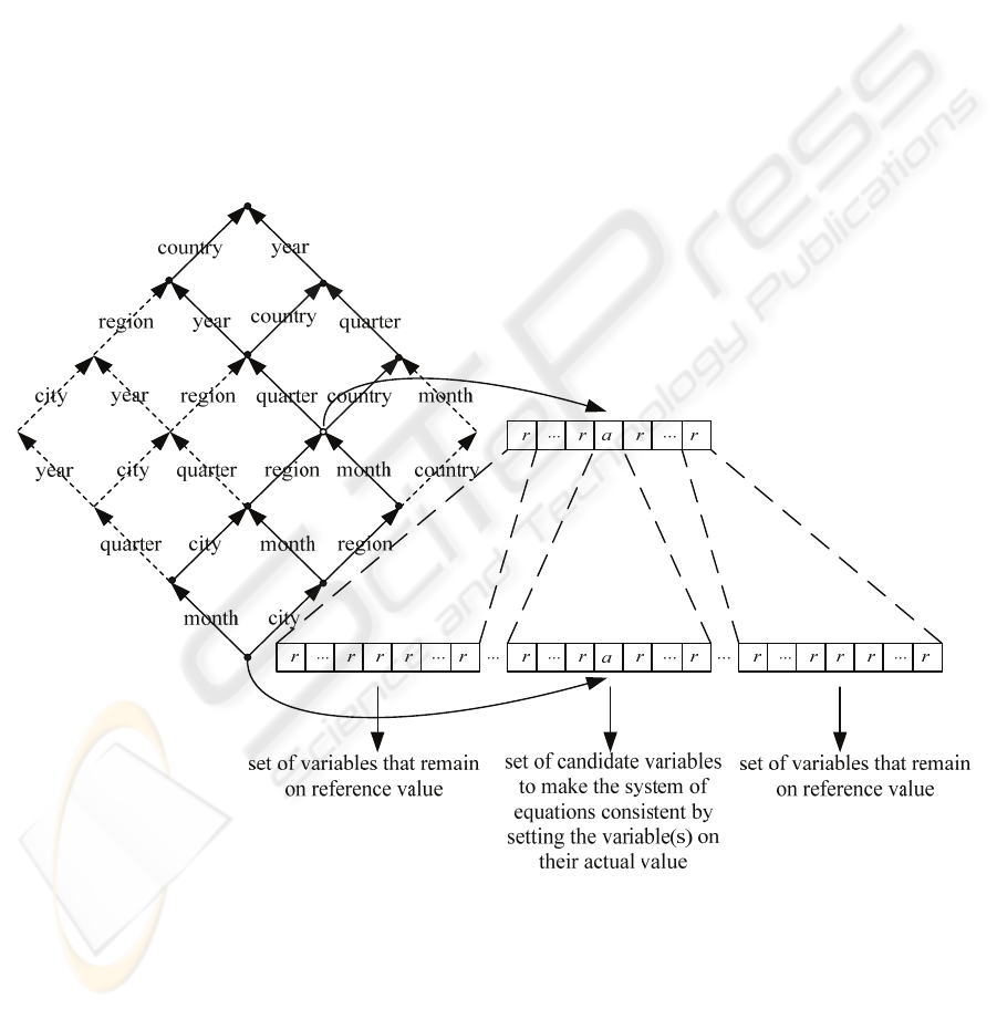
In figure 1, an illustration is given of the

working of the sensitivity analysis correction.

Suppose a business analyst changes a single instance

of the variable

y to a new actual value a while

keeping all siblings of this variable on their

reference values r. This change makes the system of

equations in the aggregation lattice inconsistent.

Now the correction procedure corrects the downsets

of instances of variable

y level by level, where

only descendants of the actual instance of

y are

considered as candidates for correction. In the last

step of the procedure the base variables are changed

accordingly to produce again a consistent system of

OLAP equations.

6 CONCLUSIONS

In this paper, we described extensions to the OLAP

framework for business analysis. Exceptional cell

values are determined based on a normative model,

often a statistical model appropriate for multi-

dimensional data. Explanation generation is

supported by the two internal structures of the

OLAP data cube: the business model and the

dimension hierarchies. Therefore, we developed a

multi-level explanation method for finding

significant causes in these structures, based on an

influence-measure which embodies a form of ceteris

paribus reasoning. This method is further enhanced

with a look-ahead functionality to detect so-called

hidden causes. The methodology as proposed uses

the concept of an explanation tree of causes, where

explanation generation is continued until a

significant contributing cause cannot be explained

further. The result of the process is a semantic tree,

where the main causes for a symptom are presented

to the analyst. Furthermore, to prevent an

information overload to the analyst, several

techniques are proposed to prune the explanation

tree.

Currently, we are working on a novel OLAP

operator that supports the analyst in answering

typical managerial questions related to sensitivity

analysis. Often the analyst wants to know how some

root variable (e.g. profit) would have been changed

if a certain lower-level successor variable (e.g. some

cost variable) is increased (ceteris paribus) with one

extra unit or one percent in the business model or

dimension hierarchy. This is related to the notion of

partial marginality and elasticity in economics. An

important related issue is that the system of

equations (e.g. a set of business model equations)

remains consistent after the influence measure is

applied on some successor variable (of the root).

Consistency in a set of OLAP equations is not trivial

because by changing a certain variable (ceteris

paribus) a (non-)linear system of equations can

become inconsistent. For instance, missing data,

dependency relations, and the presence of non-linear

relations in the business model can cause a system to

become inconsistent. It is therefore important to

investigate the criteria for consistency in the OLAP

context.

REFERENCES

E. Caron, H.A.M. Daniels, (2007). Explanation of

exceptional values in multidimensional databases.

ICSOFT 2008 - International Conference on Software and Data Technologies

246

European Journal of Operational Research, 188, 884-

897.

A.J. Feelders, “Diagnostic reasoning and explanation in

financial models of the firm”, PhD thesis, Tilburg

University (1993).

A.J. Feelders, H.A.M. Daniels, “Theory and methodolo-

gy: a general model for automated business

diagnosis”, European Journal of Operational Research,

623-637, (2001).

G. Hesslow, Explaining differences and weighting causes,

Theoria 49 (1983) 87–111.

D.C. Hoaglin, F. Mosteller, J.W. Tukey, Exploring Data

Tables, Trends and Shapes, Wiley series in

probability, New York, 1988.

P.W. Humphreys, The Chances of Explanation, Princeton

University Press, Princeton, New Jersey, 1989.

H.J. Lenz, A. Shoshani, (1997). Summarizability in OLAP

and statistical data bases, Statistical and Scientific

Database Management, 132–143.

N.S. Koutsoukis, G. Mitra, C. Lucas (1999). Adapting on-

line analytical processing for decision modelling: The

interaction of information and decision technologies,

Decision Support Systems 26 (1) 1–30.

S. Sarawagi, R. Agrawal, R. Megiddo, (1998) Discovery-

driven exploration of OLAP data cubes, in: Conf.

Proc. EDBT ’98, London, UK, pp. 168–182.

H. Scheffé, (1959) The Analysis of Variance, Wiley, New

York.

W.J. Verkooijen, (1993) Automated financial diagnosis: A

comparison with other diagnostic domains, Journal of

Information Science 19 (2), 125–135, May.

APPENDIX

Figure 1: Aggregation lattice with the dimensions Time and Location illustrating the working of the correction procedure.

EXTENSIONS TO THE OLAP FRAMEWORK FOR BUSINESS ANALYSIS

247