ESTIMATING H.264/AVC VIDEO PSNR WITHOUT REFERENCE

Using the Artiﬁcial Neural Network Approach

Martin Slanina and V

aclav

Department of Radio Electronics, Brno University of Technology, Purky

nova 118, Brno, Czech Republic

Keywords:

H.264/AVC, video quality, no reference assessment, PSNR, artiﬁcial neural network.

Abstract:

This paper presents a method capable of estimating peak signal-to-noise ratios (PSNR) of digital video se-

quences compressed using the H.264/AVC algorithm. The idea is in replacing a full reference metric - the

PSNR (for whose evaluation we need the original as well as the processed video data) - with a no reference

metric, operating on the encoded bit stream only. As we are working just with the encoded bit stream, we can

spare a signiﬁcant amount of computations needed to decode the video pixel values. In this paper, we describe

the network inputs and network conﬁgurations, suitable to estimate PSNR in intra and inter predicted pictures.

Finally, we make a simple evaluation of the proposed algorithm, having the correlation coefﬁcient of the real

and estimated PSNRs as the measure of optimality.

1 INTRODUCTION

As the video processing, storage and transmission

systems began to shift from the analog to the digital

domain, the quality assessment and evaluation meth-

ods had to be changed accordingly. For analog video,

several well deﬁned and quite easily measurable pa-

rameters sufﬁced to give a clue on the visual quality

of the video material at the consumer end. For digital

video, the visual quality at the end of the communi-

cation chain depends not only on the system charac-

teristics itself, but – to a considerable extent – on the

video content. Especially for digital video compres-

sion techniques, content is what really matters.

As the human observer is commonly the consumer

of the video material, it is his judgement that is the

ideal measure of video quality. However human ob-

servers may be and are used in the so-called subjective

quality tests, there has been a great effort to substitute

subjective assessment with an objective approach, i.e.

a technique to measure the video quality automati-

cally.

Basically, the objective approaches differ in the

extent to which the original video material is avail-

able at the quality measurement (receiver) point. In

case of full reference quality evaluation, we have full

access to the original material, which is the most de-

sirable, but at the same time the most uncommon con-

ﬁguration. If we have some limited information about

the original, we are talking about reduced reference

assessment. The worst case (and unluckily the most

common) scenario is when only the processed video,

subject to faults, compression artifacts or other degra-

dation, is available for quality assessment. What we

are trying to do is replace a full reference metric with

a no reference approach, i.e. to remove the necessity

of having the original material available.

The area of full reference metrics is quite well un-

derstood and lots of metrics have been developed to

perform quality assessment of this kind. The sim-

plest pixel-based metrics only compare the two video

sequences with simple mathematical operations (Wu

and Rao, 2006; Wang et al., 2004), while the more so-

phisticated try to make a model of the human visual

system in order to catch the most important phenom-

ena such as contrast sensitivity, masking, etc. (Win-

kler, 2005; Daly, 1992). However, although some of

the metrics perform reasonably well, the peak signal-

to-noise ratio holds its position in many application

and is still used as a performance measure.

On the other hand, the no reference video quality

assessment area has still a lot to improve. It is quite

straightforward that for no reference quality assess-

ment of a compressed video material, typical com-

pression artifacts shall be used. It is true for the com-

pression algorithms such as MPEG-2, where block ar-

tifact and blur detection can give a solid ground for

quality judgement (Fischer, 2004; Marziliano et al.,

244

Slanina M. and

Rí

cný V. (2008).

ESTIMATING H.264/AVC VIDEO PSNR WITHOUT REFERENCE - Using the Artiﬁcial Neural Network Approach.

In Proceedings of the International Conference on Signal Processing and Multimedia Applications, pages 244-250

DOI: 10.5220/0001932502440250

 SciTePress

2002). For the H.264/AVC, however, such detection

is complicated by the fact that there is an adaptive de-

blocking ﬁlter at the end of the encoding chain, which

prevents the block artifacts from appearing in the de-

compressed material. It is thus difﬁcult, if not impos-

sible, to rely on artifact detection when assessing the

H.264/AVC video. In our approach, we will use pa-

rameters describing the decoding process which are

directly present in the bit stream to feed an artiﬁ-

cial neural network. A similar approach for MPEG-2

compressed video was presented in (Gastaldo et al.,

2002).

2 PSNR AS A QUALITY

MEASURE

The peak signal-to-noise ratio is a very simple full ref-

erence quality metric. It is given by an equation (Win-

kler, 2005)

PSNR = 10log

MSE

, [dB] (1)

where m is the maximum value a pixel can take and

MSE is the mean squared error, given by

MSE =

T XY

∑

k=1

∑

i=1

∑

j=1

[ f (k, i, j) −

f (k, i, j)]

(2)

for a video sequence consisting of T frames of M × N

pixels. The symbols f (k,i, j) and

f (k, i, j) represent

the luma pixel values of the original and the distorted

video, respectively.

3 H.264/AVC ENCODING

PARAMETERS

As noted above, we will use a set of parameters

extracted from the H.264/AVC bit stream for qual-

ity assessment. In order to understand their mean-

ing, let us now brieﬂy describe the operation of an

H.264/AVC encoder. The standard describes only the

decoder (ITU-T, 2005), but the encoder conﬁguration

we will discuss is very likely to appear in most re-

alizations. A typical structure of an H.264/AVC en-

coder is shown in Fig. 1. At the input of the encoder,

we have the current frame (or ﬁeld) to be encoded and

a reference frame. The encoder maintains a list of ref-

erence frames and one or more of them may be used

for prediction. The encoder now has to decide what

type of prediction to use: Intra prediction uses only

the pixel data within the same frame, while inter pre-

diction uses different frame image data with motion

Network

Abstraction

Layer - NAL

Current

frame

Reference

frame

Motion

estimation

Motion

compensation

Intra

prediction

Filter

Reordering

QuantizationTransform

Entropy

encoder

Inverse

quantization

Inverse

transform

Reconstructed

frame

Inter prediction

Intra prediction

Figure 1: H.264/AVC encoder structure.

compensation. Furthermore, for intra as well as inter

prediction, different modes can be selected. The pre-

diction process is marked with the left oval in Fig. 1.

A mode detailed description of the available predic-

tion modes will follow in subsection 3.1

After forming the prediction, residuals remain to

be encoded. There are several transforms available

in the H.264/AVC (Richardson, 2003), whose coefﬁ-

cients are subsequently quantized and encoded in the

bit stream. More on the transform and quantization

will follow in subsection 3.2. This process is marked

with the right oval in Fig. 1.

Below the dashed line in Fig. 1, there is a return

path in the encoder. Every encoded picture is de-

coded as well, in order to provide a reference for fur-

ther prediction of subsequent pictures. This is where

the above mentioned adaptive deblocking ﬁlter can be

found, preventing the block artifacts from appearing

and making artifact detection such a difﬁcult issue for

H.264/AVC.

It is the prediction mode and the quantization

coarseness that we use for video image quality esti-

mation.

3.1 Prediction Modes

As noted above, the encoder has the option to choose

between intra and inter prediction for every mac-

roblock. Furthermore, for each of these prediction

types, there is a whole list of modes to choose from

in order to achieve the optimal quality – compression

tradeoff.

For intra prediction, each macroblock can be pre-

dicted either as one 16 × 16 block, four 8 × 8 blocks

or sixteen 4 × 4 blocks (ITU-T, 2005). Furthermore,

one special prediction mode can be used – the IPCM

mode – where no prediction is done and the pixel val-

ues are encoded directly, which may be beneﬁcial in

some situations. It should be mentioned that not all

modes are available in all encoder proﬁles. The 8 × 8

mode is, for example, only used in the high proﬁle

ESTIMATING H.264/AVC VIDEO PSNR WITHOUT REFERENCE - Using the Artificial Neural Network Approach

245

of H.264/AVC. While encoding larger blocks needs

fewer bits to signal the prediction process to the de-

coder, more energy is likely to remain in the residuals.

For example, if the encoder is limited with bit rate

constraints, it may happen that large blocks are pre-

dicted in order to spare bits even though high energy

residuals will remain for the transform.

For inter prediction, even more options are avail-

able. One macroblock may be predicted as one

16 × 16 blocks, two 16 × 8 or 8 × 16 blocks or four

8 × 8 blocks. If the 8 × 8 mode is chosen, the four

macroblock partitions may be split up in additional

four ways. There is one more mode – the direct mode

– where no additional information is transmitted and

the macroblock is simply copied from the reference

picture. Again, the predicted block size is likely to

carry a signiﬁcant amount of information on the en-

coding performance.

3.2 Quantization

In the H.264/AVC, the transform coefﬁcients are

quantized using scalar quantization. This is another

part of the encoding process, where the resulting qual-

ity can be strongly inﬂuenced. The basic forward

quantizer operation is (Richardson, 2003)

i, j

= round(Y

i, j

/Qstep), (3)

where Y

i, j

are the transform coefﬁcients, Qstep is a

quantizer step size and Z

i, j

are the quantized coefﬁ-

cients. A total of 52 Qstep values are supported by

the standard, indexed by a quantizing parameter.

We will make use of the quantizing parameter val-

ues to predict video image PSNR in section 4.

4 ESTIMATING PSNR VALUES

In the previous text, we discussed the parameters di-

rectly available in the H.264/AVC bit stream, which

may give us a clue on the quality of the decoded

video. Let us now use these parameters to develop an

algorithm capable of estimating PSNR values without

reference. For simplicity, we will only consider base-

line proﬁle to verify the correctness of our approach.

There are two important features of the baseline pro-

ﬁle we have to consider at this time – the baseline

proﬁle does not use 8 × 8 intra prediction and motion

compensated inter prediction is done only in one di-

rection, from one reference picture.

4.1 Video Sequence Set

We constructed two sets of short video sequences

in CIF resolution (352 x 288 pixels). The CIF for-

mat was selected just to verify the correctness of our

approach. Extension for other formats will then be

straightforward. One set is used for training of the

artiﬁcial neural network (training set), the other one

is used to evaluate the trained network and check

its generalization ability (evaluation set). The un-

compressed sequences are freely available (CIF Se-

quences, 2006). The two sets were constructed in or-

der to have various types of sequences (with differ-

ent spatial and temporal activity) in each of the sets.

First frames of the sequences for the test set and the

evaluation set are shown in Fig. 2 and Fig. 3, respec-

tively. Each sequence was encoded and decoded in

H.264/AVC baseline proﬁle, with four different bit

rate settings of the encoder. The VBR encoder setting

was selected, and consequently the quantizing param-

eter remained unchanged within the slices.

Figure 2: Video sequences used for network training.

Figure 3: Video sequences used for evaluation.

4.2 Intra Coded Pictures

We have already stated that for intra coded pictures,

the prediction is done only from the neighboring pix-

els within the same picture. More exactly, predic-

tion is done from image data within the same slice (a

deﬁned group of macroblocks). As we take the pre-

dicted block size as an input to our algorithm, we have

four parameters as inputs: no. of macroblocks coded

in 16 × 16 mode, no. of macroblocks coded in 8 × 8

mode, no. of macroblocks coded in 4 × 4 mode and

no. of IPCM macroblocks. We will experiment with

SIGMAP 2008 - International Conference on Signal Processing and Multimedia Applications

246

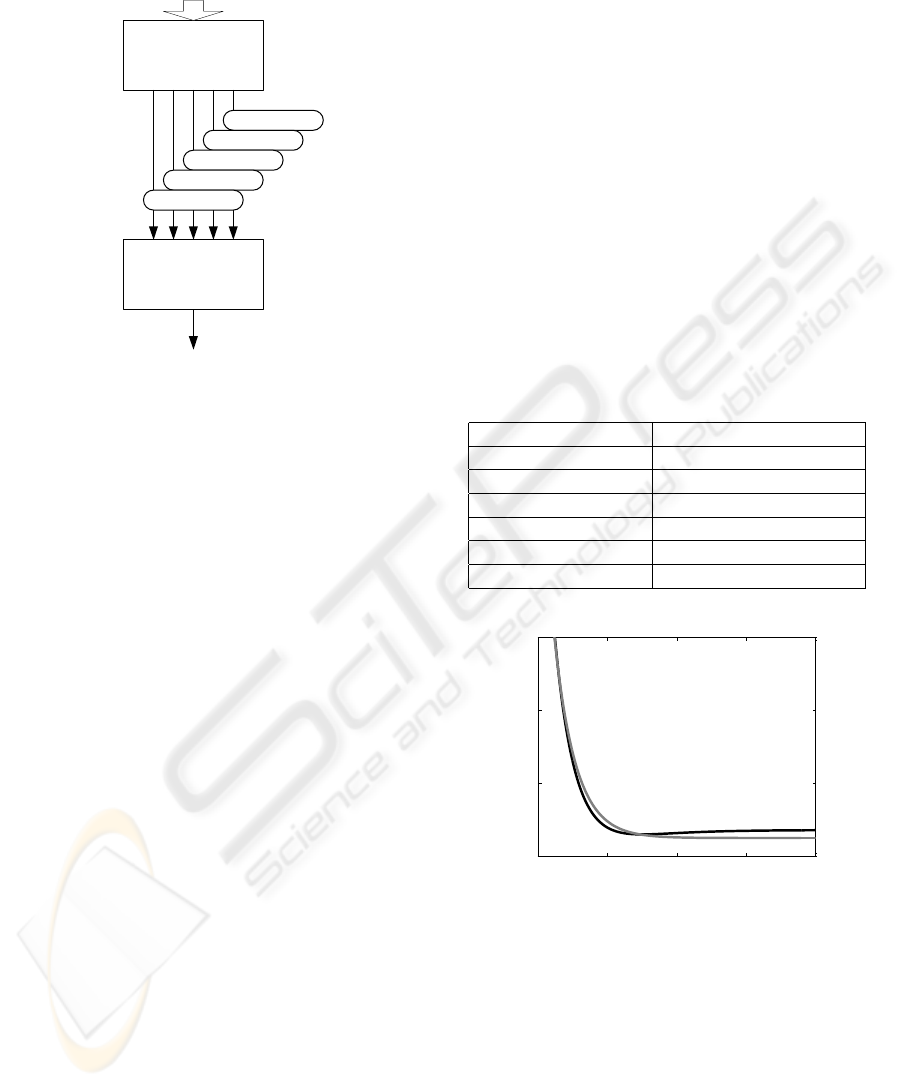
101101010000111000011101000010010011

010101010111110001101101011010010101

H.264/AVC encoded bit stream

Parameter

Extractor

16x16 blocks

8x8 blocks

4x4 blocks

IPCM blocks

Quant. par.

Artificial

Neural

Network

Estimated PSNR

Figure 4: Predicting PSNR for intra coded pictures.

artiﬁcial neural networks to estimate PSNR values us-

ing these parameters. As it is desirable to have all the

inputs normalized in the range 0 to 1 for the artiﬁcial

neural network, we divide all the values by the total

number of macroblocks within the picture. One more

input to the artiﬁcial neural network will be formed

by the quantizing parameter. Again, to stay in the

range 0 to 1, it will be divided by the factor of 52

as it is the maximum value the quantizing parameter

can take. The algorithm will then operate as shown

in Fig. 4. The scheme takes all the possible modes

into account. For the baseline proﬁle we are using,

the 8 × 8 bocks are not used and the IPCM blocks are

not likely to appear, for instance.

The ﬁrst block in the scheme is a Parameter Ex-

tractor, supposed to read the numbers of the respec-

tive prediction modes from the bit stream. For this,

we use a modiﬁed H.264/AVC reference decoder in

the version JM11 (Suehring, 2006).

4.2.1 Linear Network

As the simplest conﬁguration, we experimented with

an artiﬁcial neural network consisting of neurons with

linear transfer function only. It is known that any

feedforward conﬁguration of linear neurons can be re-

placed with an equivalent made up of a single neuron,

thus one neuron unit sufﬁces to exploit the capabilities

of linear network for our application (Bishop, 2006).

We trained the linear neuron unit on the training

set of video sequence intra frames using the gradi-

ent descent (least mean squares) algorithm (Bishop,

2006). This algorithm is designed to minimize the

mean of squared errors over the set of training exam-

ples. We used ﬁve different encoder conﬁgurations

over the ten different training sequences, resulting in

50 training examples. The training process is shown

in Fig. 5 – the graph shows how the mean squared

errors decrease for the training set with the increas-

ing training iterations (epochs) and how it develops

for the evaluation set. Fig. 6 shows how the corre-

lation coefﬁcient of the real and the estimated PSNR

changes during the training. After 2500 epochs we

reached a correlation coefﬁcient of 0.9774 for the

training set and 0.9666 for the evaluation set. The

trained network weights are listed in Table 1 for all

the input parameters scaled in the range 0 to 1. As the

IPCM and 8 × 8 blocks are not used in our conﬁgura-

tion, the corresponding weights are equal to zero. The

corresponding scatter plot diagram for the evaluation

set is shown in Fig. 7.

Table 1: Linear unit weigths for intra picture PSNR predic-

tion. Baseline proﬁle.

Input parameter Corresponding weight

Quantizing par. / 52 -47.53

IPCM blocks 0

16 × 16 blocks 26.22

8 × 8 blocks 0

4 × 4 blocks 17.37

bias 43.60

0 500 1000 1500 2000

Training epochs [-]

Mean squared error [-]

Evaluation set

Training set

Figure 5: Linear unit training.

4.2.2 Multi-Layer Network

We experimented with several conﬁgurations of

multi-layer networks as well, having a variable (1 to

5) sigmoid units in the hidden layer and one linear

unit in the output layer. The correlation coefﬁcients

we reached for the evaluation set were very close to

those achieved by the linear network. However, the

implementation of such networks is rather more com-

plex and thus in the rest of our considerations we will

only estimate PSNRs of intra predicted frames using

the linear unit as described above.

ESTIMATING H.264/AVC VIDEO PSNR WITHOUT REFERENCE - Using the Artificial Neural Network Approach

247

0 500 1000 1500 2000

0.7

0.75

0.8

0.85

0.9

0.95

Training epochs [-]

Correlation coefficient [-]

Evaluation set

Training set

Figure 6: Correlation coefﬁcient with increasing number of

training epochs.

15 20 25 30 35 40 45 50

Real PSNR [dB]

Estimated PSNR[dB]

Figure 7: Scatter plot diagram: Estimated versus real

PSNRs for intra coded pictures after 2500 training epochs

(evaluation picture set).

4.3 Inter Coded Pictures

To estimate PSNR for inter coded pictures, we will

have to consider more parameters than in the previ-

ous situation as for the inter predicted pictures more

prediction methods are available.

Intra prediction can still be used in inter predicted

pictures, so we will keep the parameters (per cent of

block types) deﬁned in section 4.2 and displayed in

Fig. 4. In addition, we will use the information of the

size of intra predicted blocks, i.e. how many blocks

were predicted with each of the available block sizes

from 16 × 16 down to 4 × 4 (see section 3.1).

As the pixel values are predicted from other pic-

tures, the PSNR of the predicted picture certainly de-

pends on the PSNR of the reference picture. There is

a whole list of pictures the H.264/AVC decoder may

use for prediction and a decision on the reference pic-

ture choice is done for each inter predicted block sep-

arately. This means the PSNR of the reference is typ-

ically changing throughout the predicted picture. Our

solution is to compute the average PSNR for each of

the inter prediction modes.

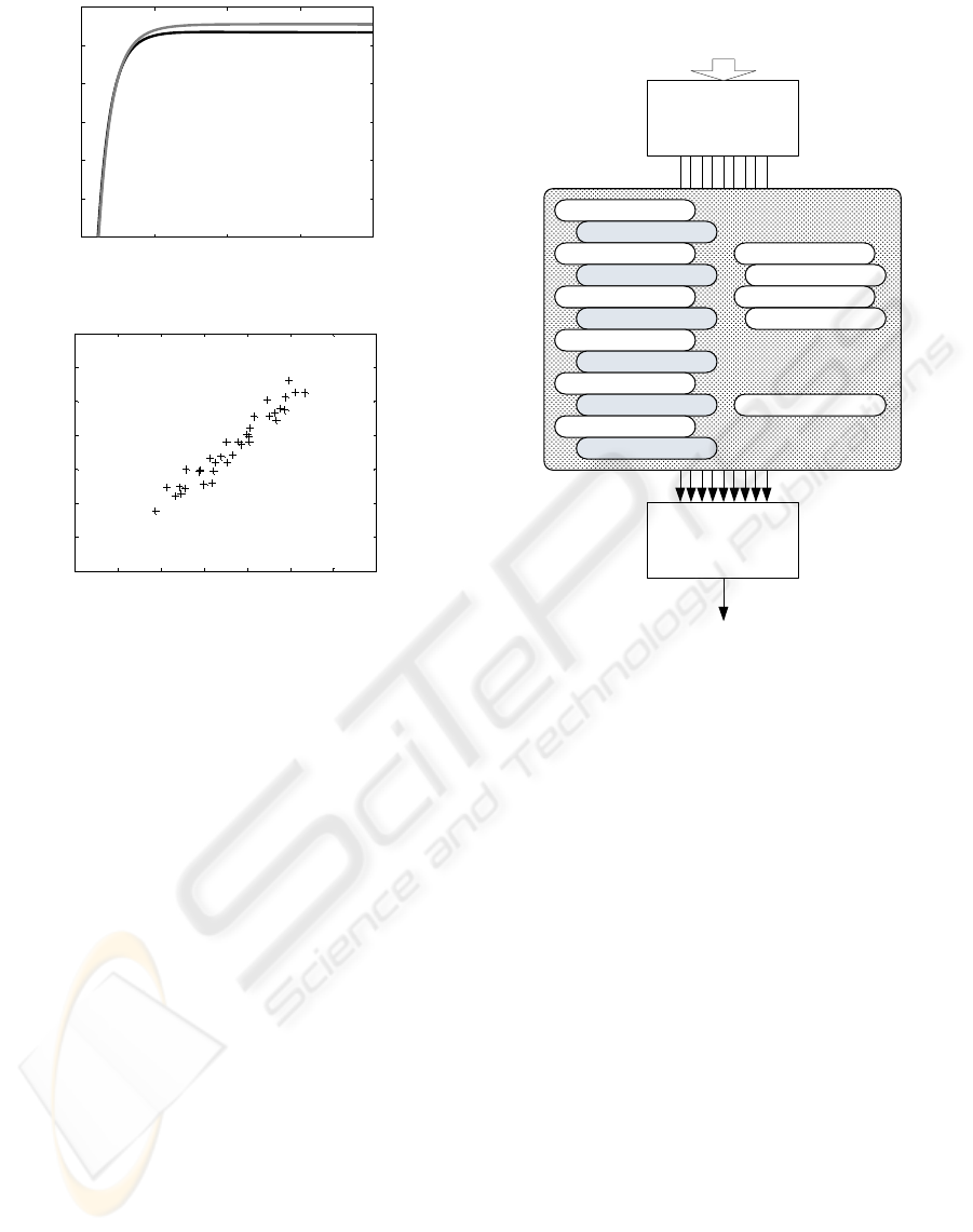
The system conﬁguration for the inter predicted

pictures is then as shown in Fig. 8. Obviously, the

101101010000111000011101000010010011

010101010111110001101101011010010101

H.264/AVC encoded bit stream

Parameter

Extractor

Artificial

Neural

Network

Estimated PSNR

16x16 intra blocks

8x8 intra blocks

4x4 intra blocks

IPCM blocks

Quant. par.

16x16 inter blocks

16x16 ref PSNR

16x8 inter blocks

16x8 ref PSNR

8x8 inter blocks

8x8 ref PSNR

8x4 inter blocks

8x4 ref PSNR

4x4 inter blocks

4x4 ref PSNR

Direct blocks

Direct ref PSNR

Figure 8: Predicting PSNR for inter coded pictures.

number of network input parameters has grown sig-

niﬁcantly.

4.3.1 Network Training

To estimate the PSNR of inter coded pictures, we tried

to use a linear network ﬁrst, similarly to the case in

section 4.2.1. However, in the case of inter predicted

pictures, the problem can not be described by a linear

network and thus the network could not be trained to

predict PSNR values correctly.

A multi-layer network is then the next choice. For

the network training, we always need the PSNR of the

reference picture the prediction is done from. In the

training process, we can still use the real PSNRs to

achieve the best performance of the trained network.

In the network performance evaluation, its own es-

timated PSNRs will be used as the refence PSNRs

(PSNR of the picture the prediction is done from).

We used four network conﬁgurations, having one

to ﬁve sigmoid (tansig) units in the hidden layer

and one linear unit in the output layer. The net-

works were trained using the backpropagation algo-

rithm with Bayesian regularization to avoid overﬁt-

ting (Bishop, 2006). The training was done for 500

epochs with a learning rate of 0.0005. We used 60

SIGMAP 2008 - International Conference on Signal Processing and Multimedia Applications

248

20 25 30 35 40 45 50

Real PSNR [dB]

Estimated PSNR [dB]

Figure 9: Scatter plot diagram: Estimated versus real

PSNRs for inter coded pictures afted 500 training epochs

(evaluation picture set).

0 10 20 30 40 50 60

Frame no.

PSNR

0 10 20 30 40 50 60

Frame no.

PSNR

Estimated

Real

Estimated

Real

Figure 10: Real and estimated PSNR for two video se-

quences (ﬁrst 60 frames).

frames of each compressed video sequence.

4.3.2 Network Performance

Fig. 9 shows the scatter plot diagram of the real end

estimated PSNRs for the ﬁrst 60 frames of the evalua-

tion set sequences each compressed with ﬁve different

conﬁgurations, the network has three sigmoid units in

the hidden layer and one linear unit in the output layer.

The correlation coefﬁcient is 0.9306.

In Fig. 10 we show how the real and estimated

PSNRs develop in time for two sequences from the

evaluation set. It is obvious the overall accuracy of

the estimation vastly depends on how exactly we are

able to estimate the PSNR of the ﬁrst (intra) frame

in the sequence. Even though PSNR for some of the

sequences was estimated quite closely, sequences re-

main in the evaluation set for which the differences

are signiﬁcant.

5 CONCLUSIONS

We have presented a method to estimate peak signal-

to-noise ratios for H.264/AVC video sequences with-

out reference. As the simplest conﬁguration, we con-

sidered H.264/AVC baseline proﬁle and worked with

low resolution video sequences.

We reached a correlation of 0.9666 for intra pre-

dicted pictures (linear network) and 0.9306 for in-

ter predicted pictures (network with 3 sigmoid units

in the hidden layer and one linear unit in the output

layer). Increasing the number of hidden units in the

network for inter PSNR prediction led to a decrease

of MSE over the training set, but also the correlation

for the evaluation set decreased.

Even though the correlation is quite high, a closer

estimate is still desired as the PSNR is a logarithmic

measure and even a few decibel differences may rep-

resent quite big differences in quality.

The network weights and biases are only learned

for a certain encoder implementation. When migrat-

ing to a system using a different encoder, the networks

should be trained again for the given encoder.

Our considerations were limited to the baseline

proﬁle only. For other proﬁles, bi-directional predic-

tion has to be taken into account and the PSNR of the

reference pictures has to be included in the estimation

process.

ACKNOWLEDGEMENTS

This paper was ﬁnancially supported by the Czech

Grant Agency under grant No. 102/08/H027 ”Ad-

vanced methods, structures and components of elec-

tronics wireless communication” and by the research

program MSM 0021630513 ”Electronic Communica-

tion Systems and Technologies of New Generation”

(ELCOM).

REFERENCES

Bishop, C. M. (2006). Pattern Recognition and Machine

Learning. Springer, New York. ISBN 0-387-31073-8.

CIF Sequences (2006). [online]. Retrieved December 2006

from http://trace.eas.asu.edu/yuv/cif.html.

Daly, S. J. (1992). The visible difference predictor: an al-

gorithm for the assessment of image ﬁdelity. In Proc.

SPIE: Human Vision, Visual Processing, and Digital

Display III, volume 1666, pages 2–15.

Fischer, W. (2004). Digital Television: A Practical Guide

for Engineers. Springer, Berlin. ISBN 3-540-01155-2.

ESTIMATING H.264/AVC VIDEO PSNR WITHOUT REFERENCE - Using the Artificial Neural Network Approach

249

Gastaldo, P. et al. (2002). Objective assessment of MPEG-

2 video quality. Journal of Electronic Imaging,

11(3):365–374.

ITU-T (2005). Recommendation H.264. Advanced video

coding for generic audiovisual services. The Interna-

tional Telecommunication Union, Geneva.

Marziliano, P. et al. (2002). A no-reference perceptual blur

metric. In Proceedings of the International Confer-

ence on Image Processing, volume 3, pages 57–60.

Richardson, I. E. G. (2003). H.264 and MPEG-4 Video

Compression. Wiley, Chichester (England). ISBN 0-

470-84837-5.

Suehring, K. (2006). The h.264/MPEG-4 AVC reference

software – jm11. [online]. Retrieved November 2006

from http://iphome.hhi.de/suehring/tml/download/.

Wang, Z., Lu, L., and Bovik, A. C. (2004). Video qual-

ity assessment based on structural distortion measure-

ment. Signal Processing: Image Communication,

19(2):121–132.

Winkler, S. (2005). Digital Video Quality: Vision Models

and Metrics. Wiley, Chichester. ISBN 0-470-02404-6.

Wu, H. R. and Rao, K. R. (2006). Digital Video Image Qual-

ity and Perceptual Coding. Taylor & Francis, Boca

Raton. ISBN 0-8247-2777-0.

SIGMAP 2008 - International Conference on Signal Processing and Multimedia Applications

250