ACCURACY ANALYSES OF PASSIVE TRACKING OF SEVERAL

CLICKING SPERM WHALES

A Case of Complex Sources Binding

Fr´ed´eric Caudal and Herv´e Glotin

System & Information Sciences Laboratory (LSIS - UMR CNRS 6168), Universit´e du Sud Toulon Var

BP 20132, 83957 La Garde Cedex, France

Keywords:

Delay estimation, marine mammals, acoustic tracking, Cram´er-Rao Lower Bound, acoustic propagation.

Abstract:

This paper provides a real-time passive underwater acoustic method to track multiple emitting whales using

four or more omni-directional widely-spaced bottom-mounted hydrophones and to evaluate the performance

of the system via the Cram´er-Rao Lower Bound (CRLB) and Monte Carlo simulations. After a non-parametric

Teager-Kaiser-Mallat signal ﬁltering, rough Time Delays Of Arrival are calculated, selected and ﬁltered, and

used to estimate the positions of whales for a constant or linear sound speed proﬁle. The complete algorithm

is tested on real data from the NUWC and the AUTEC. The CRLB and Monte Carlo simulations are computed

and compared with the tracking results. Our model is validated by similar results from the US Navy and

Hawaii univ labs in the case of one whale, and by similar whales counting from the Columbia univ. ROSA

lab in the case of multiple whales. At this time, our tracking method is the only one giving typical speed and

depth estimations for multiple (5) emitting whales located at 1 to 5 km from the hydrophones.

1 INTRODUCTION

Processing of Marine Mammal (MM) signals for pas-

sive oceanic acoustic localization is a problem that

has recently attracted attention in scientiﬁc litera-

ture and in some institutes like the AUTEC

and

the NUWC

. Motivation for processing MM signals

stems from increasing interest in the behavior of en-

dangered MM

. One of the goals of current research

in this ﬁeld is to develop tools to localize the vocal-

izing and clicking whale for species monitoring. In

this paper we propose a low cost time-domain track-

ing algorithm based on passive acoustics. The exper-

iments of this paper consist in tracking an unknown

number of sperm whales (Physeter catodon). Clicks

are recorded on two datasets of 20 and 25 minutes

on a open-ocean widely-spaced bottom-mounted hy-

drophone array. The output of the method is the

track(s) of the MM(s) in 3D space and time. In Sec-

tion 2 we brieﬂy review studies of source separation

methods and the main characteristics of MM signals

and we propose a real-time algorithm for MM tran-

Atlantic Undersea Test & Evaluation Center - Bahamas

Naval Undersea Warfare Center of the US Navy

This work is founded by the ”Conseil r´egional

Provence-Alpes-Cˆote d’Azur” France, and partly by Chrisar

Software Inc.

sient call localization. In Section 3, we recall brieﬂy

the CRLB (Kay, 1993) and the conﬁdence ellipses

theory. In Section 4 we show and compare results of

tracks estimates with results from specialized teams

and the performance system with the CRLB.

2 PROBLEM FORMULATION

This papers deals with the 3D tracking of MM using

a widely-spaced bottom-mounted array in deep wa-

ter. It focuses on sperm whale clicks; detection and

classiﬁcation are not a concern. There were previous

algorithms developed in the state of art (Giraudet and

Glotin, 2006b; Giraudet and Glotin, 2006a; Nosal and

Frazer, 2006; Morrissey et al., 2006) but none are able

to have satisfying results for multiple tracks. Most of

them are far from being real-time. The main goal is

to build a robust and real-time tracking model, despite

ocean noise, multiple echoes, imprecise sound speed

proﬁles, an unknown number of vocalizing MM, and

the non-linear time frequency structure of most MM

signals. Background ocean noise results from the ad-

dition of several noises: sea state, biological noises,

ship noise and molecular turbulence. Propagation

characteristics from an acoustic source to an array of

Caudal F. and Glotin H. (2008).

ACCURACY ANALYSES OF PASSIVE TRACKING OF SEVERAL CLICKING SPERM WHALES - A Case of Complex Sources Binding.

In Proceedings of the International Conference on Signal Processing and Multimedia Applications, pages 55-62

DOI: 10.5220/0001933700550062

 SciTePress

hydrophones include multipath effects (and reverber-

ations), which create secondary peaks in the Cross-

Correlation (CC) function that the generalized CC

methods cannot eliminate.

2.1 Material

Table 1: Hydrophones positions: D=Datasets,

Dist=Distance to barycenter (m).

D Hydros Dist X (m) Y (m) Z (m)

H 1 5428 18501 9494 -1687

H 2 4620 10447 4244 -1677

H 3 2514 14119 3034 -1627

H 4 1536 16179 6294 -1672

H 5 3126 12557 7471 -1670

H 6 4423 17691 1975 -1633

H 7 1518 10658 -14953 -1530

H 8 4314 12788 -11897 -1556

H 9 2632 14318 -16189 -1553

H 10 3619 8672 -18064 -1361

H 11 3186 12007 -19238 -1522

The signals are records from the ocean ﬂoor near An-

dros Island - Bahamas (Tab.1), provided with celer-

ity proﬁles and recorded in March 2002. Datasets

are sampled at 48 kHz and contain MM clicks and

whistles, background noises like distant engine boat

noises. Dataset1 (D1) is recorded on hydrophones

1 to 6 with 20 min length while dataset2 (D2)

is recorded on hydrophones 7 to 11 with 25 min

length. We will use a constant sound speed with

c = 1500ms

−1

or a linear proﬁle with c(z) = c

+ gz

where z is the depth, c

= 1542ms

−1

is the sound

speed at the surface and g = 0.051s

−1

is the gradi-

ent. Sound source tracking is performed by continu-

ous localization in 3D using Time Delays Of Arrival

(T) estimation from four hydrophones.

2.2 Signal Filtering

A sperm whale click is a transient increase of sig-

nal energy lasting about 20 ms (Fig.1-a). Therefore,

we use the Teager-Kaiser (TK) energy operator on the

discrete data:

Ψ[x(n)] = x

(n) − x(n+ 1)x(n− 1), (1)

where n denotes the sample number. An important

property of TK is that it is nearly instantaneous given

that only three samples are required in the energy

computation at each time instant. Considering the raw

signal s(n) as:

s(n) = x(n) + u(n),

where x(n) is the signal of interest (clicks), u(n) is an

additive noise deﬁned as a process realization consid-

ered wide sense stationary (WSS) Gaussian during a

short time, by applying TK to s(n), Ψ[s(n)] is:

Ψ[s(n)] ≈ Ψ[x(n)] + w(n),

where w(n) is a random gaussian process (Kandia

and Stylianou, 2006). The output is dominated by

the clicks energy. Then, we reduce the sampling

frequency to 480Hz by the mean of 100 adjacent

bins to reduce the variance of the noise and the data

size. We apply the Mallat’s algorithm (Mallat, 1989)

with the Daubechies wavelet (order 3). We chose

this wavelet for its great similarity to the shape of

a decimated click (Giraudet and Glotin, 2006b; Gi-

raudet and Glotin, 2006a). The signal is denoised

with a universal thresholding (Donoho, 1995) deﬁned

as D(u

,λ) = sgn(u

)max(0,|u

| − λ), with u

the

wavelet coefﬁcients, λ =

(2log

(Q))σ

, and Q

the length of the signal resolution level to denoise.

The noise standard deviation σ

is calculated on each

10s window on the raw signal with a maximum like-

lihood criterion. σ

is the standard deviation of the

wavelet coefﬁcients on a resolution level of a gener-

ated, reduced and 0-mean Gaussian noise. This ﬁl-

tering step is very fast without any parameter. Fig.1-

d is the ﬁltered signal on multiple (Fig.1-c) emitting

MMs.

2.3 Rough

T Estimation

First, T estimates are based on MM click realignment

only. Every 10s, and for each pair of hydrophones

(i, j), the difference between times t

and t

of the ar-

rival of a click train on hydrophones i and j is referred

as T(i, j) = t

−t

. Its estimate

T(i, j) is calculated by

CC of 10s chunks (2s shifting) of the ﬁltered signal

for hydrophones i and j (Giraudet and Glotin, 2006b;

Giraudet and Glotin, 2006a). We keep the 35 high-

est peaks on each CC to determine the corresponding

T(i, j). The ﬁltered signals give a very fast rough esti-

mate of T (precision ± 2ms). Fig.(1.e) shows the CC

with the raw signal and (1.f) with the ﬁltered signal.

Without ﬁltering, CC generates spurious delays esti-

mates and the tracks are not correct. The maximum

T rank (Fig.2) in D1, pitching the source localization,

are high among the 35

T kept in the CC which justi-

ﬁes this number.

2.4

T Selection and Localization with a

Constant Proﬁle

Each signal shows echoes for each click (Fig.1 b),

maybe due to the reﬂection of the click train off the

SIGMAP 2008 - International Conference on Signal Processing and Multimedia Applications

2.32 2.33 2.34 2.35 2.36 2.37 2.38 2.39

−0.4

−0.2

0.2

0.4

Time of recording (s)

2 4 6 8 10

−0.5

0.5

Time of recording (s)

4 6 8 10 12

−0.5

0.5

Time of recording (s)

−8 −6 −4 −2 0 2 4 6 8

−10

4 6 8 10 12

0.5

Time of recording (s)

−8 −6 −4 −2 0 2 4 6 8

CC: delay estimation

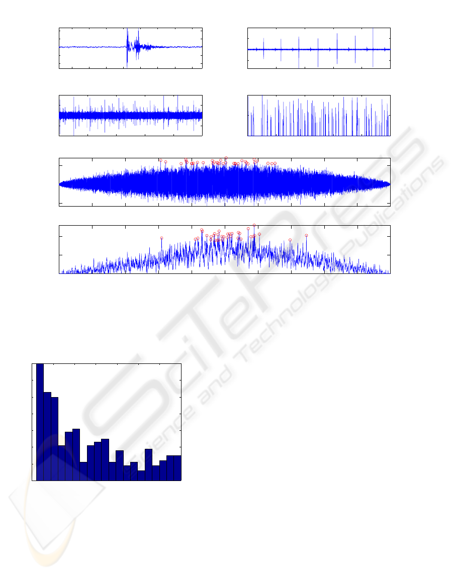
Figure 1: (a): Detail of a click. (b): raw signal (D2) of hydrophone 7 (H7) during the ﬁrst 10s of recording, containing 7

clicks and their echoes. (c): raw signal (D1) of H3 during the ﬁrst 10s of recording showing multiple emissions. (d): (c) after

ﬁltering. (e): CC between (c) and corresponding raw signal chunk of H1. (f): idem than (e) but with (d). Circles correspond

to the 35 maximum peaks.

0 5 10 15 20 25 30 35

Number of

Maximum

T rank

Figure 2: Maximum

T rank histogram in the CC for each

triplet.

ocean surface or bottom or different water layers. We

use a method based on autocorrelation (Giraudet and

Glotin, 2006b; Giraudet and Glotin, 2006a) to elimi-

nate it. Then, thanks to the

T transitivity system de-

scribed in (Giraudet and Glotin, 2006b) we keep

triplets coming from the same source. Finally, thanks

to the measured delays and an acoustic model based

on a constant sound speed proﬁle, the least squares

cost function determines the MM positions using a

multiple non linear regression with Gauss-Newton

method (Levenberg-Marquardt)(Giraudet and Glotin,

2006b). The residuals are approximatively following

a Chi-square distribution with Nc− d degrees of free-

dom, noted X

Nc−d

, Nc is the number of hydrophones

couples considered and d the number of unknowns,

here 3 (x,y,z). The position is accepted if the residual

is inferior to a threshold x, That is calculated solving

P = prob(X

Nc−d

> x) with P = 0.01 (we keep 99% of

the estimates).

2.5 Source Localization with a Linear

Sound Speed Proﬁle

It is well known that the ray paths in a medium with

linear sound speed proﬁle are arcs of circles and fur-

ther the radius of the circle can be computed (Fig.3).

is the sound speed at the source, θ

is the launch

angle of the ray at the source, measured relatively to

the horizontal. From the geometry shown in Fig.3, the

center of the circle, (xc,zc), along which the ray path

is an arc, is (White et al., 2006):

ACCURACY ANALYSES OF PASSIVE TRACKING OF SEVERAL CLICKING SPERM WHALES - A Case of

Complex Sources Binding

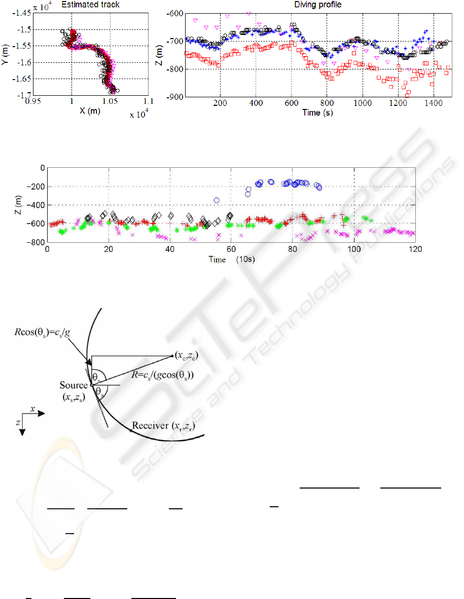
Figure 4: Plan view and diving proﬁle of the MM in D2, our estimates with a linear (A) (Caudal and Glotin, 2008) or constant

proﬁle (2); and estimates from Morrissey’s (Morrissey et al., 2006) (▽) and from Nosal’s (Nosal and Frazer, 2006) methods

(o).

Figure 5: Averaged diving proﬁle in D1. Each symbol corresponds to one whale in Fig.6 (Bottom to top (+), (o), (A), (x),

(⋄)).

Figure 3: Geometry for a source and receiver in a linear

proﬁle (White et al., 2006).

+ x

− z

)

2(x

− x

)

− z

= z

−

(2)

For linear sound speed proﬁle the course time τ of

the ray is:

τ =



log



− z



− log



R+ x

− x

R+ x

− x



. (3)

Using Eqs.(2)-(3) allows one to compute the propaga-

tion time from the source to any receiver and then the

whale position.

3 THE CRLB AND CONFIDENCE

REGIONS

3.1 The CRLB

The CRLB provides the maximum acurracy for the

estimation of the position. Considering a constant

sound speed proﬁle, the function model of the TDOA

is deﬁned:

s(θ) =







∑

k=1

i,k

− θ

)

−

∑

k=1

j,k

− θ

)







where X

{

i, j}

is the vector coordinate of hy-

drophone {i, j}, θ is the unknown parameters vec-

tor [x y z]

and c

the celerity. Thus, considering the

TDOA noise Gaussian and B its variance-covariance

matrix, the Fisher Information matrix is:

= ∇

s(θ)B

−1

∇

s(θ).

Then, the CRLB is B

= I

−1

SIGMAP 2008 - International Conference on Signal Processing and Multimedia Applications

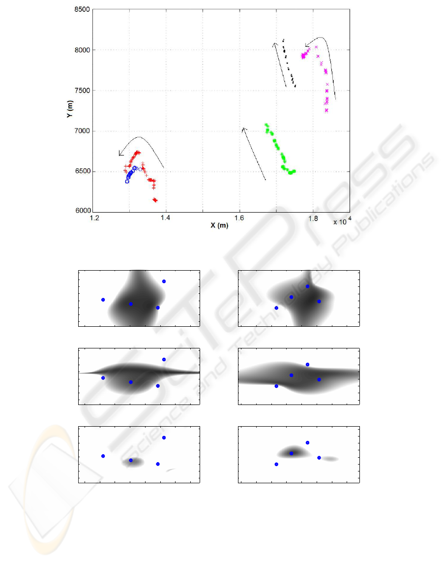
Figure 6: Plan view in D1. Each symbol corresponds to one of the 5 whales. The arrows stress the directions.

X (m)

Y (m)

0.8 1 1.2 1.4 1.6 1.8 2 2.2

x 10

−2000

2000

4000

6000

8000

10000

12000

X (m)

Y (m)

0.8 1 1.2 1.4 1.6 1.8 2 2.2

x 10

−2000

2000

4000

6000

8000

10000

12000

X (m)

Y (m)

0.8 1 1.2 1.4 1.6 1.8 2 2.2

x 10

−2000

2000

4000

6000

8000

10000

12000

H10

X (m)

Y (m)

0.4 0.6 0.8 1 1.2 1.4 1.6 1.8

x 10

−2.2

−2

−1.8

−1.6

−1.4

−1.2

−1

−0.8

x 10

H10

X (m)

Y (m)

0.4 0.6 0.8 1 1.2 1.4 1.6 1.8

x 10

−2.2

−2

−1.8

−1.6

−1.4

−1.2

−1

−0.8

x 10

H10

X (m)

Y (m)

0.4 0.6 0.8 1 1.2 1.4 1.6 1.8

x 10

−2.2

−2

−1.8

−1.6

−1.4

−1.2

−1

−0.8

x 10

Figure 7: CRLB values scaled in gray colors with a plan view: black means a null CRLB and white a CRLB≥10 m. For all

the ﬁgures, a depth of 500m was chosen. (A): CRLB on x values, dataset D1. (B): y, D1. (C): z, D1. (D): x, D2. (E): y, D2.

(F): z, D2.

3.2 Conﬁdence Regions

The conﬁdence ellipse generalizes the notion of con-

ﬁdence interval in case of gaussian vector in two di-

mensions. Considering a stochastic gaussian vector

X ∼ N(µ,Σ) of two dimensions with Σ > 0. We have

to determine the level curves of the gaussian distribu-

tionl, i.e. the points x of the ellipse

(x− µ)

∗

−1

(x− µ) = r

ACCURACY ANALYSES OF PASSIVE TRACKING OF SEVERAL CLICKING SPERM WHALES - A Case of

Complex Sources Binding

Being a symmetrical positive matrix, Σ can be

spectraly factorized as Σ = PDP

∗

where P is the or-

thonormal matrix of the eigen vectors and D the diag-

onal matrix of the eigen values. For each x, the point ˜x

is deﬁned with ˜x = D

−1/2

Px, then | ˜x|

= r, i.e. all the

˜x is the circle centered with radius r : ˜x(ρ) = r[cos(ρ)

sin(ρ)]

∗

for 0 ≤ ρ < 2π. The parametric equation of

the ellipse is:

x(ρ) = µ+ rP

∗

1/2



cos(ρ)

sin(ρ)



,0 ≤ ρ < 2π

The quadratic norm of the stochastic vector

X =

−1/2

PX is distributed with the chi-square distribu-

tion with 2 degrees of freedom. Putting r = 5.99, then

P(X ∈ x ∈ R

: (x− µ)

∗

−1

(x− µ) ≤ r) = 0.95

This means the real position is 95% likely to be inside

the ellipse.

4 RESULTS

4.1 Tracking Comparisons

For D2 (Fig.4), a constant and a linear sound speed

proﬁle were used (Caudal and Glotin, 2008) and the

results are similar with the Morrissey’s (Morrissey

et al., 2006) and Nosal’s (Nosal and Frazer, 2006)

methods. The diving proﬁle underlines a bias of about

50 to 100m between the linear and the constant pro-

ﬁles results, emphasizing the importance of the cho-

sen proﬁles. Moreover with the linear sound speed,

the results are about the same as Morrissey’s and

Nosal’s, who used proﬁles corresponding to the pe-

riod and place of the recordings. Results on D1 are

shown in Fig.6-5 for a linear sound speed proﬁle. We

thus localize 5 MM. The conﬁdence regions are com-

puted for the two datasets with a Monte Carlo method.

The ellipses maxima (30m) ﬁt with MM length (20m).

4.2 CRLB Computation

The CRLB provide the maximum acurracy for the lo-

calization. Here, we computed the CRLB (in me-

ter) in the space (x,y,z) and plot the values for both

datasets (Fig.7). We consider that the standard devi-

ation of the noise is equal to the quantiﬁcation noise

with a sampling frequency of 480Hz. The main de-

pendencies of the bounds are the noise and the array

conﬁguration.

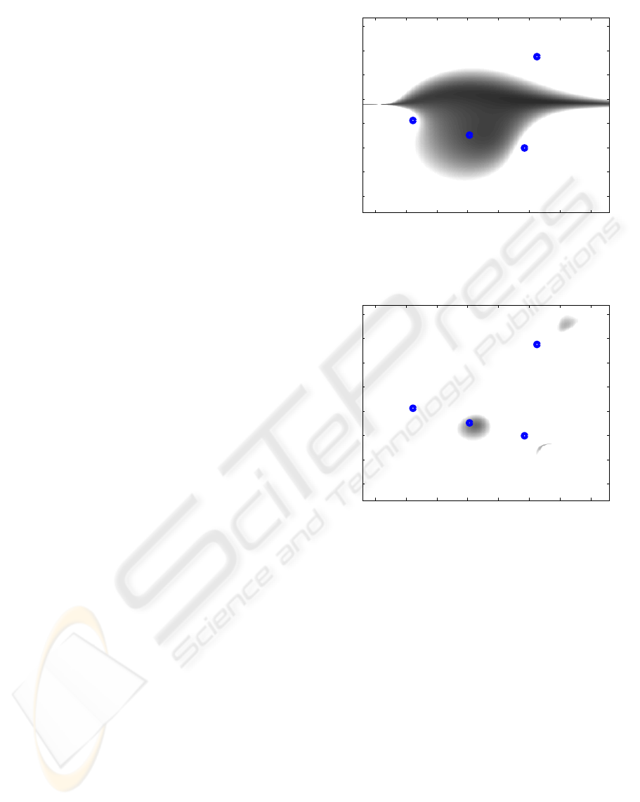
In ﬁgures 8 and 9, the CRLB on y and z is shown

for a depth of 1000m, and is just about the same for

X (m)

Y (m)

0.8 1 1.2 1.4 1.6 1.8 2 2.2

x 10

−2000

2000

4000

6000

8000

10000

12000

Figure 8: CRLB on y axis, plan view, dataset D1,

depth=1000m.

X (m)

Y (m)

0.8 1 1.2 1.4 1.6 1.8 2 2.2

x 10

−2000

2000

4000

6000

8000

10000

12000

Figure 9: CRLB on z axis, plan view, dataset D1,

depth=1000m.

a depth of 500m. Thus, as the mean depth of a sperm

whale is in this range, the CRLB likewise.

4.3 The Conﬁdence Regions

We apply a Monte Carlo method with a gaussian dis-

tribution noise with the standard deviation described

above. For each

T realization, the source position

is calculated. We deduce the variance and the mean

for each position to plot the conﬁdence regions with

a conﬁdence level of 0.95, which means that there

is 0.95 probability for the whale to be in the ellipse

centered on the position. In D2, the mean values of

the conﬁdence intervals on X, Y, Z axes are about

18, 16 and 30 m (Fig.10). This justiﬁes the decima-

tion on the raw signal, because the error on X and

Y axes are close to the sperm whale length (20m).

The results conﬁrm that the errors on the vertical axis

SIGMAP 2008 - International Conference on Signal Processing and Multimedia Applications

1.02 1.03 1.04 1.05

x 10

−1.6

−1.58

−1.56

−1.54

x 10

X (m)

Y (m)

1.03 1.04 1.05 1.06

x 10

−1.67

−1.66

−1.65

−1.64

x 10

X (m)

Y (m)

−1.68−1.66−1.64−1.62 −1.6

x 10

−800

−750

−700

Y (m)

Z (m)

−1.59−1.58−1.57−1.56−1.55

x 10

−800

−750

−700

−650

Y (m)

Z (m)

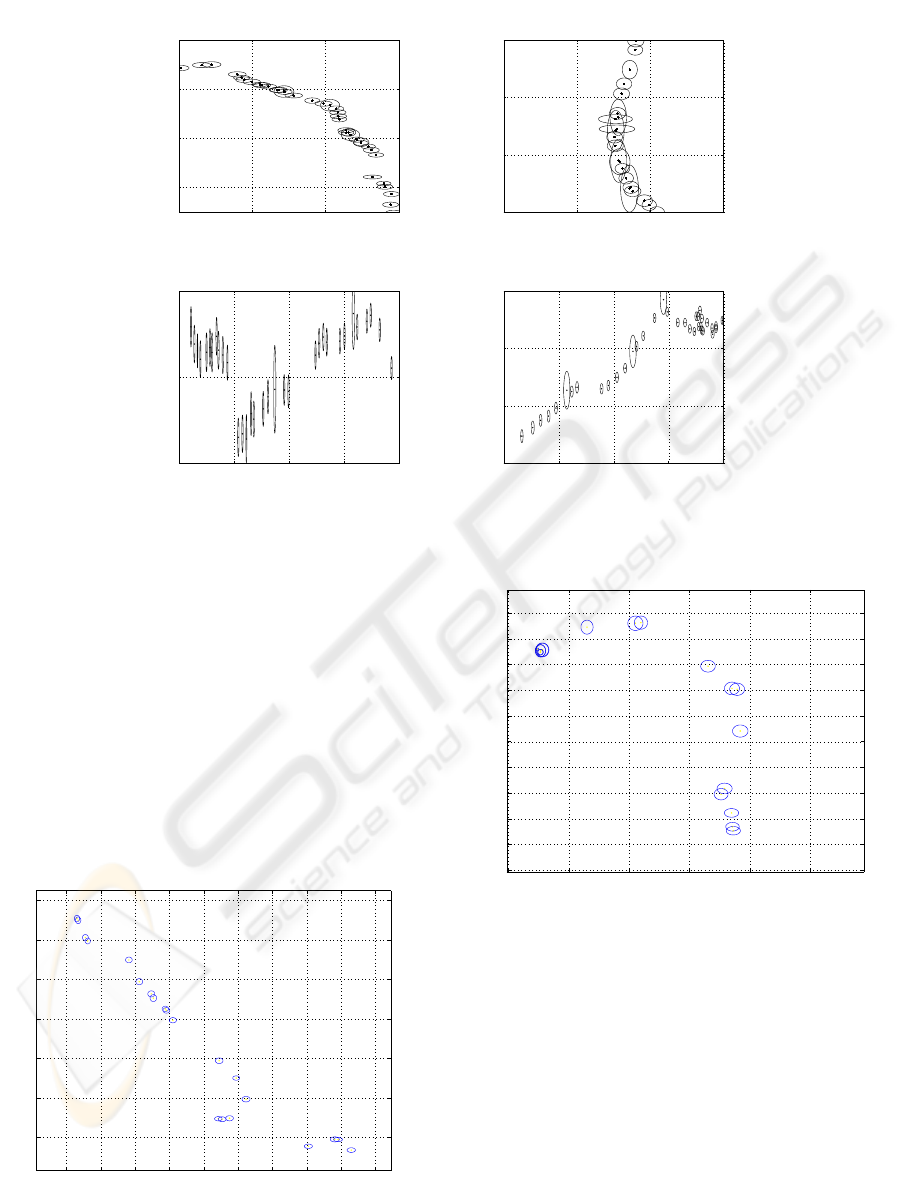
Figure 10: Conﬁdence regions projection on X and Y and on Z and Y axes for D2 trajectory.

are meaningfully higher than the other axes because

the distance between each hydrophones in this direc-

tion (maximum difference on the Z axis between hy-

drophones is 200m) is smaller. The D1 results ob-

tained with a linear proﬁle (Fig.6), indicate ﬁve tra-

jectories. The farthest whales in D1 from the hy-

drophones array center have a larger uncertainty with

an error of about 20 to 30m on X and Y axes (Fig.12),

while the whales close to the center (Fig.11) exhibit

an error of about 10 to 20m like for D2 (Fig.6). Those

uncertainties are reasonable according to the sperm

whale length.

1.67 1.68 1.69 1.7 1.71 1.72 1.73 1.74 1.75 1.76

x 10

6500

6600

6700

6800

6900

7000

7100

X (m)

Y (m)

Figure 11: Conﬁdence regions projection on X and Y for

the whale in the middle (* symbol), D1 trajectory.

1.76 1.78 1.8 1.82 1.84 1.86

x 10

7000

7100

7200

7300

7400

7500

7600

7700

7800

7900

8000

X (m)

Y (m)

Figure 12: Conﬁdence regions projection on X and Y for

the whale in the right (x symbol), D1 trajectory.

4.4 Performance Comparisons

Comparing the CRLB and the ellipses, we denote the

correlation between maximum accuracy and conﬁ-

dence regions. Figures 7-C and 7-F show the accuracy

on z axis is ≥10 m for both datasets in the tracking

regions which is consistent with the ellipses results.

The CRLB (in D1, ﬁgures 6-D,E) also explains that

the farthest whale has larger conﬁdence regions. But

for both datasets, the CRLB on x and y is far inferior

to 10m inside the array whereas our ellipses are about

10 to 20m. Maybe other parameters like the approxi-

ACCURACY ANALYSES OF PASSIVE TRACKING OF SEVERAL CLICKING SPERM WHALES - A Case of

Complex Sources Binding

mated celerity proﬁle are involved in.

5 CONCLUSIONS

The tracking algorithm presented in this paper is real-

time on a standard laptop and works for one or mul-

tiple emitting sperm whales. Depth results with con-

stant speed contains a bias errors due to the refraction

of the sound paths from the MM to the receivers what

a linear speed corrects. An other way to tackle the

speed proﬁle issue (Glotin et al., 2008) is to estimate it

as a fourth unknown in the regression. Our algorithm

has no species dependency as long as it processes

all transients. At this time, only our algorithm gives

results with typical speed and depth estimations for

multiple emitting whales. In D2, results indicate that

only one sperm whale was present in the area, unless

other whales in the area were quiet during the selected

25-min period. Moreover, according to ROSA Lab es-

timation based on click clustering, averaged number

of MM for each 5min chunks on D1 is [4.3;5.3;4;3.6]

(Halkias and Ellis, 2006) similar to ours ([4;4;4;3]).

The localization accuracy is computed via the CRLB

and the conﬁdence ellipses which are correct consid-

ering the MM length. The high depth error is mainly

due to the low precision reachable with the CRLB

considering the array conﬁguration. Our method pro-

vides thus robust online detecting/counting system of

clicking MM in open ocean.

REFERENCES

Caudal, F. and Glotin, H. (2008). Multiple real-time 3d

tracking of simultaneous clicking whales using hy-

drophone array and linear sound speed proﬁle. In

ICASSP IEEE, volume 4p.

Donoho, D. L. (1995). De-noising by soft thresholding.

IEEE Trans. IT, 41:613–627.

Giraudet, P. and Glotin, H. (2006a). Echo-robust and real-

time 3d tracking of marine mammals using their tran-

sient calls recorded by hydrophones array. In ICASSP

IEEE.

Giraudet, P. and Glotin, H. (2006b). Real-time 3d tracking

of whales by echo-robust precise tdoa estimates with a

widely-spaced hydrophone array. Applied Acoustics,

67:1106–1117.

Glotin, H., Caudal, F., and Giraudet, P. (2008). Whales

cocktail party: a real-time tracking of multiple whales.

International Journal Canadian Acoustics, page 7p.

Halkias, X. and Ellis, D. (2006). Estimating the number

of marine mammals using recordings form one micro-

phone. In ICASSP IEEE.

Kandia, V. and Stylianou, Y. (2006). Detection of sperm

whale clicks based on the teager-kaiser energy opera-

tor. Applied Acoustics, 67:1144–1163.

Kay, S. (1993). Fundamentals of statistical signal process-

ing. PTR.

Mallat, S. (1989). A theory for multiresolution signal de-

composition: The wavelet representation. volume 11,

pages 674–693. IEEE Transaction on Pattern Analysis

and Machine Intelligense.

Morrissey, R., Ward, J., DiMarzio, N., Jarvisa, S., , and

Moretti, D. (2006). Passive acoustics detection and lo-

calization of sperm whales in the tongue of the ocean.

Applied Acoustics, 62:1091–1105.

Nosal, E. and Frazer, L. (2006). Delays between direct and

reﬂected arrivals used to track a single sperm whale.

Applied Acoustics, 62:1187–1201.

White, P., Leighton, T., Finfer, D., Powles, C., and Bau-

mann, O. (2006). Localisation of sperm whales

using bottom-mounted sensors. Applied Acoustics,

62:1074–1090.

SIGMAP 2008 - International Conference on Signal Processing and Multimedia Applications