NOISE REDUCTION BASED ON CROSS TF ε-FILTER

Tomomi Abe

Major in Pure and Applied Physics, Waseda university 55N-4F-10A, 3-4-1 Okubo, Shinjuku-ku, Tokyo, 169-8555, Japan

Mitsuharu Matsumoto, Shuji Hashimoto

Department of Applied Physics, Waseda university 55N-4F-10A, 3-4-1 Okubo, Shinjuku-ku, Tokyo, 169-8555, Japan

Keywords:

Noise reduction, speech enhancement, ε-ﬁlter, time-frequency domain.

Abstract:

A time-frequency ε-ﬁlter (TF ε-ﬁlter) is an advanced ε-ﬁlter applied to complex spectra along the time axis. It

can reduce most kinds of noise while preserving a signal that varies frequently such as a speech signal. The

ﬁlter design is simple and it can effectively reduce noise. It is applicable not only to small amplitude stationary

noise but also to large amplitude nonstationary noise. However when we consider the noise that varies much

frequently along the time axis, TF ε-ﬁlter cannot reduce noise without the signal distortion. When we consider

the noise where the neighboring frequency bins have similar powers such as impulse noise, we can reduce the

noise by using ε-ﬁlter applied to the complex spectra not along the time axis, but along the frequency axis.

This paper introduces an advanced method for noise reduction that applies ε-ﬁlter to complex spectra not only

along the time axis but also along the frequency axis labeled cross TF ε-ﬁlter. We conducted the experiments

utilizing the sounds with stationary, nonstationary and natural noise.

1 INTRODUCTION

Noise reduction plays an important role in speech

recognition and individual identiﬁcation. When

we consider the instruments like hearing-aids and

phones, noise reduction for a monaural sound is

strongly expected. It will also be easy to miniatur-

ize the system size because it requires only one sig-

nal. The spectral subtraction (SS) is a well-known ap-

proach for reducing the noise signal of the monaural-

sound (Boll, 1979). It can reduce the noise effectively

despite of the simple procedure. However, it can han-

dle only the stationary noise. It also needs to estimate

the noise in advance. Although noise reduction uti-

lizing Kalman ﬁlter has also been reported (Kalman,

1960; Fujimoto and Ariki, 2002), the calculation cost

is large. Some authors have reported a model based

approach for noise reduction (Daniel et al., 2006).

In this approach, we can extract the objective sound

by learning the sound model in advance. However,

it is not applicable to the signals with the unknown

noise as well as SS. There are some approaches uti-

lizing comb ﬁlter (Lim et al., 1978). In this approach,

we ﬁrstly estimate the pitch of the speech signal, and

reduce the noise signal utilizing comb ﬁlter. How-

ever, the estimation error results in the degradation

of the speech quality. Some authors have reported

the method utilizing ε-ﬁlter (Harashima et al., 1982;

Arakawa et al., 2002). ε-ﬁlter is a nonlinear ﬁlter,

which can reduce the noise signal with preserving the

signal. ε-ﬁlter is simple and has some desirable fea-

tures for noise reduction. It does not need to have the

model not only of the signal but also of the noise in

advance. It is easy to be designed and the calculation

cost is small. It can reduce not only the stationary

noise but also the nonstationary noise. However, it

can reduce only the small amplitude noise in princi-

ple. To solve the problems, the method labeled TF

ε-ﬁlter was proposed (Abe et al., 2007). TF ε-ﬁlter

is an improved ε-ﬁlter applied to the complex spec-

tra along the time axis in time-frequency domain. By

utilizing TF ε-ﬁlter, we can reduce not only small am-

plitude stationary noise but also large amplitude non-

stationary noise. However TF ε-ﬁlter cannot reduce

the noise without distortion when the noise changes

frequently along the time axis such as impulse noise.

To solve the problem, we apply ε-ﬁlter to complex

spectra not only along the time axis but also along the

105

Abe T., Matsumoto M. and Hashimoto S. (2008).

NOISE REDUCTION BASED ON CROSS TF -FILTER.

In Proceedings of the International Conference on Signal Processing and Multimedia Applications, pages 105-112

DOI: 10.5220/0001935001050112

 SciTePress

frequency axis labeled cross TF ε-ﬁlter. By apply-

ing ε-ﬁlter to the complex spectra along the two axes,

we can reduce the noise even if it changes frequently

along the time axis. It need not estimate the noise as

well as TF ε-ﬁlter in advance. We also show the ex-

perimental results of the proposed method compared

to the other methods such as SS and TF ε-ﬁlter.

2 NOISE REDUCTION

UTILIZING TD ε-FILTER AND

TF ε-FILTER

To clarify the problems of a time-domain ε-ﬁlter

(TD ε-ﬁlter)(Harashima et al., 1982; Arakawa et al.,

2002), we ﬁrstly explain the TD ε-ﬁlter algorithm. Let

us deﬁne x(k) as the input signal at time k. Let us also

deﬁne y(k) as the output signal of the ε-ﬁlter at time k

as follows:

y(k) = x(k) +

∑

i=−P

a(i)F(x(k+ i) − x(k)), (1)

where a(i) represents the ﬁlter coefﬁcient. a(i) is usu-

ally constrained as follows:

∑

i=−P

a(i) = 1. (2)

The window size of the ε-ﬁlter is 2P+ 1. F(x) is the

nonlinear function described as follows:

|F(x)| ≤ ε

: −∞ ≤ x ≤ ∞, (3)

where ε

is a constant. This method can reduce small

amplitude noise while preserving the speech signal.

For example, we can set the nonlinear function F(x)

as follows:

F(x) =



x (−ε

≤ x ≤ ε

)

0 (otherwise).

(4)

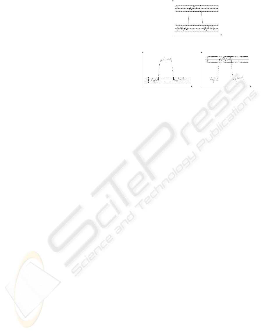
Figure 1 shows the basic concept of an ε-ﬁlter

when Eq.4 is utilized as F(x). Figure 1(a) shows the

waveform of the input signal.

Executing the ε-ﬁlter at point A in Figure 1(a), we

ﬁrst replace all the points where the distance from A

is larger than ε

by the value of point A. We then

summate the signals in the same window. Figure 1(b)

shows the basic concept of this procedure. The dotted

line represents the points where the distance from A

is larger than ε

. In Figure 1(b), the continuous line

represents the values replaced through this procedure.

As a result, if the points are far from A, the points are

ignored. On the other hands, if the points are close to

A, the points are smoothed. Due to this procedure, the

ε0

(a) Input signal

(b) When a TD ε-filter

is applied to the point A

Amplitude

Time

is applied to the point B

Amplitude

Time

Amplitude

Time

Figure 1: The basic concept of a TD ε-ﬁlter.

ε-ﬁlter reduces noise while preserving the precipitous

attack and decay of the speech signal. In the same

way, by executing the ε-ﬁlter at point B in Figure 1(a),

we replace all the points where the distance from B is

larger than ε

by the value of the point B. The points

are ignored if they are far from B, while the points

are smoothed if the points are close to B as shown in

Figure 1(c). Consequently, we can reduce small am-

plitude noise near by the processed point while pre-

serving the speech signal.

An ε-ﬁlter can reduce small amplitude noise in the

time domain. However, due to the procedure, it is

not applicable to large amplitude noise. To solve this

problem, Time-Frequency ε-ﬁlter (TF ε-ﬁlter) was

proposed (Abe et al., 2007). TF ε-ﬁlter utilizes the

distribution difference of the speech signal and the

noise in the frequency domain. The following as-

sumptions regarding the sound sources are used:

• Assumption 1. Speech signal has greater vari-

ation in power than noise signal in the time-

frequency domain.

• Assumption 2. Noise signal is distributed more

uniformly and with less variation in the time-

frequency domain.

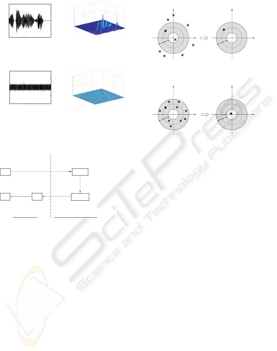
Figure 2 depicts the speech signal and the white noise

signal in the time and the time-frequency domains.

As shown in Figure 2, assumptions 1 and 2 are

fulﬁlled in the case of various noise like white noise

and natural noise such as the sound of a cooling fan.

In Figures 2(b) and (d), the power is normalized using

the maximal power of the speech signal. When we

consider frequency bins where there are signals, the

ratio of noise power to signal power is smaller than

the ratio of noise amplitude to signal amplitude in the

time domain. In TF ε-ﬁlter, we utilize this feature to

SIGMAP 2008 - International Conference on Signal Processing and Multimedia Applications

106

0 1 2

-0.4

-0.2

0.2

0.4

Time[s]

Amplitude

(a)

Speech signal

(in time domain)

Time[s]

Power

0.5

x 10

Frequency[Hz]

(b)Speech signal

(in time-frequency domain)

0 1 2

-0.4

-0.2

0.2

0.4

Time[s]

Amplitude

(c)

Noise signal

(in time domain)

Power

Frequency[Hz]

Time[s]

0.5

x 10

(d) Noise signal

(in time-frequency domain)

Figure 2: A speech signal or noise signal in the time and

frequency domains.

)

STFT

V (

)

y(k)

ISTFT

Time domain

Time-frequency domain

(2)

(1)

(4)

TF ε-filter

along the frequency axis

)

(3)

v(k)

TD ε-filter

Figure 3: Block diagram of combining TF ε-ﬁlter and TD

ε-ﬁlter.

apply an ε-ﬁlter to high-level noise.

Figure 3 illustrates the method combining TF ε-

ﬁlter and TD ε-ﬁlter with a block diagram. As shown

in Figure 3(1), we ﬁrstly transform the input signal

x(k) to the complex amplitude X(κ, ω) by short term

Fourier transformation(STFT) as follows:

X(κ, ω) =

∞

∑

l=−∞

x(κ+ l)W(l)e

− jωl

, (5)

where W, κ and ω represent the window function, the

time frame in the time-frequency domain and the an-

gular frequency, respectively. j represents the imag-

inary unit. Next we execute a TF ε-ﬁlter, which is

an ε-ﬁlter applying to complex spectra along the time

axis in the time-frequency domain, as shown in Fig-

ure 3(2). In this procedure, V(κ, ω) is obtained as

follows:

V(κ, ω) =

∑

i=−Q

a(i)X

′

(κ+ i, ω), (6)

Im Im

εF

(a) Speech signal

εF

(b) Noise signal

Figure 4: Differences in performance when a TF ε-ﬁlter is

applied to the speech signal and noise.

where the window size of ε-ﬁlter is 2Q+ 1,

′

(κ+ i, ω) (7)











X(κ, ω)

(||X(κ, ω)| − |X(κ+ i, ω)|| > ε

)

X(κ + i, ω)

(||X(κ, ω)| − |X(κ+ i, ω)|| ≤ ε

)

and ε

is a constant.

Figure 4 illustrates the differences in performance

when we apply a TF ε-ﬁlter to the speech signal and

the noise. The horizontal axis and the vertical axis

represent the real axis and the imaginary axis, respec-

tively. In Figure 4, ∗ and × represent the processed

point and the other signal points in the same win-

dow, respectively. Point A in Figure 4(a) and point

B in Figure 4(b) represent the complex amplitude of

the processed point. A

′

and B

′

represent the complex

amplitudes of the outputs when we apply the TF ε-

ﬁlter to the points A and B, respectively. Executing

the TF ε-ﬁlter, we ﬁrstly replace the complex ampli-

tude of the signal outside of the shadow area by that

of A. We then summate the complex spectra of all

the points in the same window. Due to handling com-

plex spectra, when we have many signals that have

similar amplitudes but different phases, the real part

and imaginary part cancel each other. In other words,

even if the amplitude of the noise is large, the noise

is reduced because they cancel each other. Note that

the noise is reduced not only when the amplitude of

NOISE REDUCTION BASED ON CROSS TF e-FILTER

107

the noise is small but also when the amplitude of the

noise is large because of this procedure. Figure 4(a)

represents the basic concept in the case that the power

varies drastically like a speech signal. When we con-

sider a signal whose power varies frequently, the dif-

ference between the absolute value of A and that of

the other signals is large as shown in Figure 4(a). For

this reason, many signals in the same window as the

point A are replaced by A. As a result, when we han-

dle the speech signal, the complex amplitude of the

processed point is intact. Figure 4(b) represents the

basic concept in case that the power does not vary so

much like a noise signal. When we consider a noise

signal, the difference between the absolute value of B

and that of the other signals is relatively small com-

pared with the speech signal. Hence, few signals in

the same window as point B are replaced by B. In

other words, when handling noise, the complex am-

plitude of the processed point becomes smaller when

the TF ε-ﬁlter is applied. Based on these aspects, we

can reduce noise while preserving the signal by set-

ting ε

appropriately.

Hence, the TF ε-ﬁlter is effective even when the

power of the noise to signal is large. Additionally,

under assumption 2, the TF ε-ﬁlter becomes more ef-

fective. When assumption 2 is satisﬁed, the variation

of the noise to the signal in the frequency domain be-

comes smaller than that in the time domain. As a con-

sequence, even if the noise varies frequently in the

time domain, the ε-ﬁlter can be applied in the time-

frequency domain.

Next, we transform V(κ, ω) to v(k) by inverse

STFT as shown in Figure 3(3).

To reduce the remaining noise, we additionally ap-

ply the ε-ﬁlter in the time domain to v(k) as shown in

Figure 3(4). Note that the ε-ﬁlter in the time domain

can be utilized because large amplitude noise has al-

ready been reduced in the previous procedure. The

output y(k) can be obtained as follows:

y(k) =

∑

i=−P

a(i)v

′

(k+ i), (8)

where

′

(k+ i) =



v(k) (|v(k + i) − v(k)| > ε

)

v(k+ i) (|v(k+ i) − v(k)| ≤ ε

)

(9)

and ε

is a constant.

3 NOISE REDUCTION

UTILIZING CROSS TF

ε-FILTER

TF ε-ﬁlter can reduce the various types of noise ef-

fectively. However, when we use the noise that varies

much frequently along the time axis, TF ε-ﬁlter can-

not reduce noise without the signal distortion. When

we consider the noise where the neighboring fre-

quency bins have similar powers such as impulse

noise, we can reduce the noise by using ε-ﬁlter ap-

plying to complex spectra not along the time axis, but

along the frequency axis.

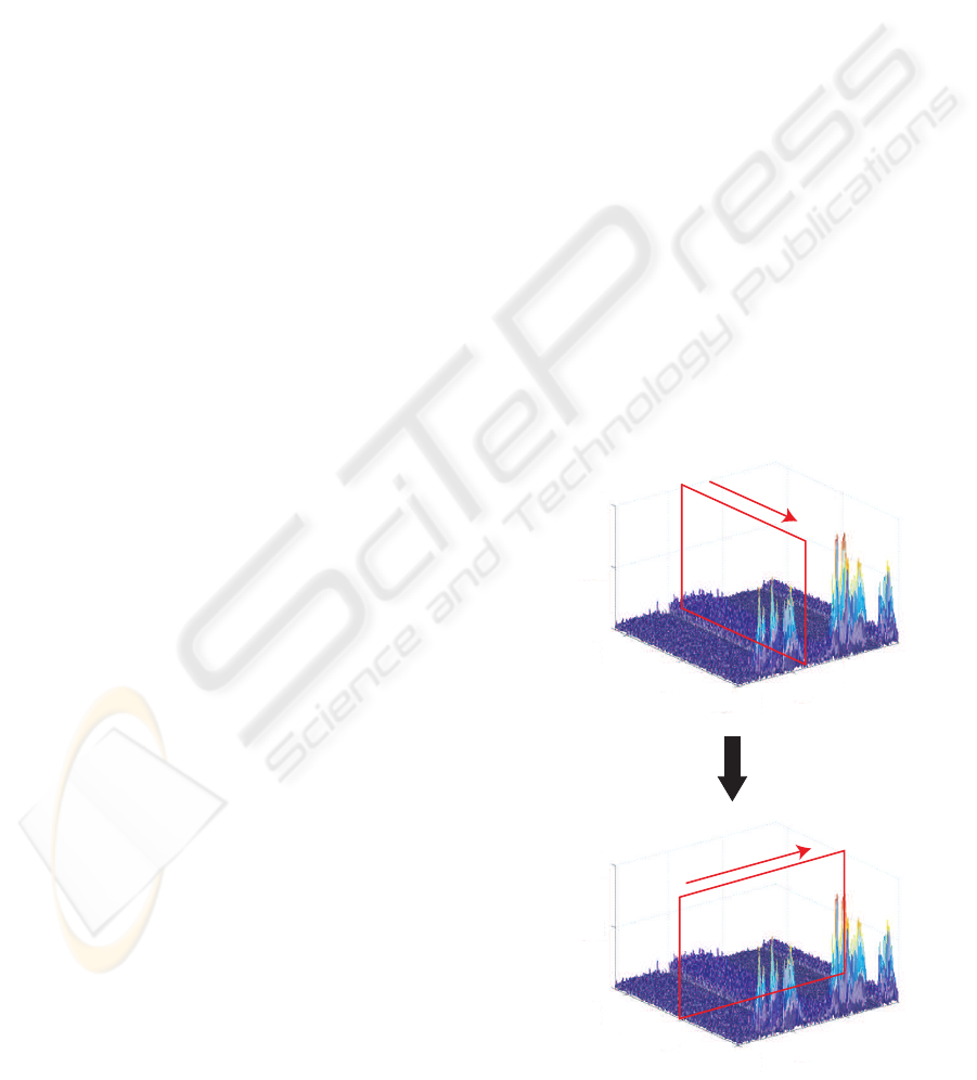
Figure 5 shows the basic concept of the proposed

method. At ﬁrst, as shown in Figure 5 “Step 1”, we

apply the ε-ﬁlter to the complex spectra along the fre-

quency axis to reduce the noise where the neighboring

frequency bins have similar power although the noise

amplitude varies drastically such as the impulse noise

and white noise whose amplitude varies. Next we ap-

ply ε-ﬁlter to complex spectra along the time axis to

reduce the noise that distributes wider than the speech

signal in the frequency domain as shown in Figure 5

“Step 2”.

Figure 6 illustrates the proposed method with a

filtering

Frequency[Hz]

Time[s]

filtering

Frequency[Hz]

Time[s]

0.5

x 10

0.5

x 10

Figure 5: The basic concept of cross TF ε-ﬁlter.

SIGMAP 2008 - International Conference on Signal Processing and Multimedia Applications

108

)

STFT

U (

)

y(k

)

ISTFT

Time domain Time-frequency domain

)

(2)

(1)

(4)

ε-filter applying

to complex spectra

along the frequency axis

)

ε-filter applying

to complex spectra

along the time axis

(3)

Figure 6: The block diagram of the proposed method.

block diagram. Let us consider x(k), and X(κ, ω)

transformed from x(k) by STFT as well as Eq.5 as

shown in Figure 6(1). Next we apply ε-ﬁlter to com-

plex spectra along the frequency axis as shown in Fig-

ure 6(2). In this procedure, U(κ, ω) is obtained as fol-

lows:

U(κ, ω) =

∑

i=−N

a(i)X

′

(κ+ i, ω), (10)

where

′

(κ+ i, ω) (11)











X(κ, ω)

(||X(κ, ω)| − |X(κ, ω+ i)|| > ε

)

X(κ, ω + i)

(||X(κ, ω)| − |X(κ, ω+ i)|| ≤ ε

is a constant and 2N + 1 is window size. Then we

employ ε-ﬁlter applying to complex spectra along the

time axis as shown in Figure 6(3). In this procedure,

Y(κ, ω) is obtained as follows:

Y(κ, ω) =

∑

i=−M

a(i)U

′

(κ+ i, ω), (12)

where

′

(κ+ i, ω) (13)











U(κ, ω)

(||X(κ, ω)| − |X(κ+ i, ω)|| > ε

)

U(κ + i, ω)

(||X(κ, ω)| − |X(κ+ i, ω)|| ≤ ε

is a constant and 2M + 1 is the window size. Next

we transform Y(κ, ω) to y(k) by inverse STFT as

shown in Figure 6(4). We label this process “cross

TF ε-ﬁlter”.

4 EXPERIMENT

4.1 Experimental Condition

We conducted the experiments utilizing a speech sig-

nal with a noise signal. As the speech signal, we uti-

Table 1: Common parameters.

Parameter Value

Sampling frequency 44100

STFT Block size

512

Hop size 256

Window function

Hanning window

lized “Japanese Newspaper Article Sentences” edited

by the Acoustical Society of Japan. We also prepared

three kinds of noise signals: stationary noise, nonsta-

tionary noise and natural noise. The signal and the

noise are mixed in the computer. To compare the ef-

fectiveness of the proposed method to other methods,

we conducted the experiments utilizing three meth-

ods; spectral subtraction (SS), the method combining

TF ε-ﬁlter and TD ε-ﬁlter and cross TF ε-ﬁlter. Table

1 shows the value of common parameters for all the

experiments.

To evaluate the performance of noise reduction,

we use signal-to-noise ratio (SNR) and signal-to-

distortion ratio (SDR). SNR is deﬁned as follows:

SNR = 10· log







∑

k=1

s(k)

∑

k=1

n(k)







, (14)

where s(k), n(k) and L represent the speech signal at

time k, the noise signal at time k, and the length of the

signal, respectively. To calculate SNR of the output

signal, we separately applied each method to the sig-

nal and noise, and calculated the output SNR by using

the obtained signal and noise. SDR can be represented

as follows:

SDR = 10 · log







∑

k=1

(k)

∑

k=1

(k) − s

out

(k))







, (15)

where s

(k) and s

out

(k) represent the input signal and

the output signal at time k respectively, when we used

only the speech signal. SDR represents how much the

signal is distorted by reducing the noise. Through-

out all the experiments, the parameters of SS and the

method combining TF ε-ﬁlter and TD ε-ﬁlter are set

optimally. On the other hand, in cross TF ε-ﬁlter, ε

was set at 0.1. We only change ε

depending on the

noise to show the robustness concerning the param-

eter setting although we can reduce the noise more

effectively. SNR of the input signal is set at 10[dB]

throughout all of the experiments.

NOISE REDUCTION BASED ON CROSS TF e-FILTER

109

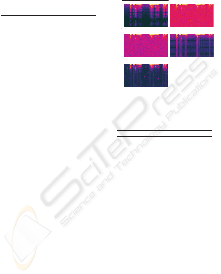
Table 2: SNR and SDR when a signal with stationary noise

is utilized.

SNR[dB] SDR[dB]

Input signal 10.0 —

SS 18.3 21.7

TD ε-ﬁlter processed

after TF ε-ﬁlter 40.6 18.9

Cross TF ε-ﬁlter 44.4 19.3

4.2 Experimental Results in the Case of

Stationary Noise

We ﬁrst conducted the experiment utilizing a signal

with stationary noise. We prepared a speech signal

and white noise as the signal and the stationary noise,

respectively. We set ε

in the proposed method at

0.7. We also set the window size of ε-ﬁlter applied to

complex spectra in the proposed method along the fre-

quency axis and the time axis at 101 and 11, respec-

tively. Table 2 shows the results of the experiments

for stationary noise.

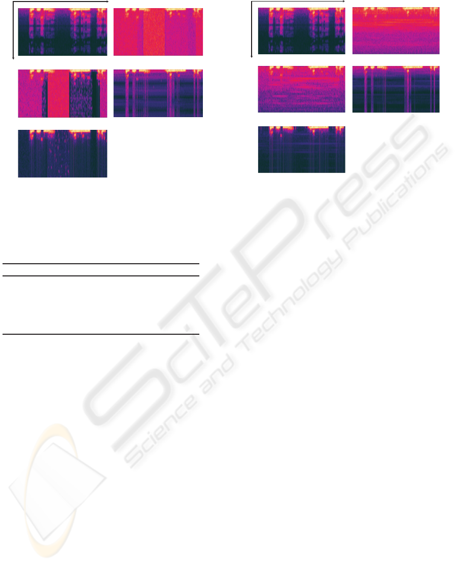
As shown in Table 2, the proposed method could

reduce the noise compared to the other methods with

preserving the signal. Figure 7 shows the sound spec-

trograms. In Figure 7, bright color represents that the

signal power is high while dark color represents that

the signal power is low. Figure 7(a) shows the spec-

trogram of the original signal. Figure 7(b) shows the

spectrogram of the signal with stationary noise. Fig-

ures 7(c)-(e) show the spectrograms of the output of

SS, the output of the method combining TF ε-ﬁlter

and TD ε-ﬁlter and the output of the proposed method,

respectively. As shown in Figure 7, when we used the

proposed method, the noise could be reduced more

effectively than the other methods.

4.3 Experimental Results in the Case of

Nonstationary Noise

The experiment was conducted using a signal with

nonstationary noise. We used the same speech sig-

nal as in Sec.4.2. We prepared white noise with an

amplitude that sometimes varied. We set ε

in the

proposed method at 1.1. We also set the window size

of ε-ﬁlter applied to complex spectra in the proposed

method along the frequency axis and the time axis

81 and 11, respectively. Table 3 shows the results of

the experiments on nonstationary noise. As shown

in Table 3, the SNR of the proposed method is supe-

rior to those of the other methods. Figure 8(a) shows

the spectrogram of the original signal. Figure 8(b)

shows the spectrogram of the signal with nonstation-

(a) Original signal (b) Input signal

(e) Cross TF ε-filter

Time

Frequency

(d) TF and TD ε-filter

Figure 7: Experimental results when a signal with station-

ary noise is utilized.

Table 3: SNR and SDR when a signal with nonstationary

noise is utilized.

SNR[dB] SDR[dB]

Input signal 10.0 —

SS 15.5 21.9

TD ε-ﬁlter processed

after TF ε-ﬁlter 40.8 16.3

Cross TF ε-ﬁlter 44.2 17.3

ary noise. Figures 8(c)-(e) show the spectrograms of

the outputs of SS, the output of the method combining

TF ε-ﬁlter and TD ε-ﬁlter and the output of the pro-

posed method, respectively. The relation between the

color and signal power is the same as in Sec.4.2. As

shown in Figure 8, when we use the proposed method,

the noise could be reduced more effectively than the

other methods even if we use the nonstationary noise

as noise.

4.4 Experimental Results in the Case of

Natural Noise

To evaluate the performance of the proposed method

for natural noise, we conducted the experiment uti-

lizing a speech signal and a noise generated from

the cooling fan of a personal computer. The most

power of noise used in this experiment is distributed

in the low-frequency range. We set ε

in the proposed

method at 1.8. We also set the window size of ε-ﬁlter

applied to complex spectra in the proposed method

along the frequency axis and the time axis 51 and 11,

SIGMAP 2008 - International Conference on Signal Processing and Multimedia Applications

110

(a) Original signal (b) Input signal

(e) Cross TF ε-filter

Time

Frequency

(d) TF and TD ε-filter

Figure 8: Experimental results when a signal with nonsta-

tionary noise is utilized.

Table 4: SNR and SDR when a signal with natural noise is

utilized.

SNR[dB] SDR[dB]

Input signal 10.0 —

SS 17.4 20.1

TD ε-ﬁlter processed

after TF ε-ﬁlter 38.2 13.4

Cross TF ε-ﬁlter 40.2 15.0

respectively. Table 4 shows the results of the experi-

ments for natural noise. As shown in Table 4, the SNR

of the proposed method is superior to those of the

other methods as well as in the case of stationary noise

and nonstationary noise. Figure 9(a) shows the spec-

trogram of the original signal. Figure 9(b) shows the

spectrogram of the signal with natural noise. Figures

9(c)-(e) show the spectrograms of the outputs of SS,

the output of the method combining TF ε-ﬁlter and

TD ε-ﬁlter and the output of the proposed method, re-

spectively. The relation between the color and signal

power is the same as in Sec.4.2. As shown in Figure

9, when we use the proposed method, the noise could

be reduced more effectively than the other methods

even if the natural noise was used as noise.

5 CONCLUSIONS

In this paper, we introduced an algorithm for noise re-

duction applying ε-ﬁlter to complex spectra not only

along the time axis but also along the frequency axis

in time-frequency domain. The proposed method can

(a) Original signal (b) Input signal

(e) Cross TF ε-filter

Time

Frequency

(d) TF and TD ε-filter

Figure 9: Experimental results when a signal with natural

noise is utilized.

reduce not only stationary noise but also nonstation-

ary and natural noise effectively with preserving sig-

nal clarity. The experimental results showed that the

proposed method could be applied to various kinds of

noise. The proposed method could reduce the louder

noise compared with the conventional methods such

as the method combining TF and TD ε-ﬁlter and SS.

It is considered that the proposed method can be ap-

plied not only to the speech in Japanese but also to

the speech in English with noise because the perfor-

mance of the proposed method depends on only the

power change of speech and noise signal. For future

works, we would like to conﬁrm the robustness of the

proposed method for various input SNR and various

types of noise. We also aim to determine each param-

eter adaptively.

ACKNOWLEDGEMENTS

This research was supported by the research grant

of Support Center for Advanced Telecommunica-

tions Technology Research (SCAT), by the research

grant of Tateisi Science and Technology Founda-

tion, and by the Ministry of Education, Science,

Sports and Culture, Grant-in-Aid for Young Scien-

tists (B), 20700168, 2008. This research was also

supported by Waseda University Grant for Special

Research Projects(B), No.2007B-142, No.2007B-143

and No.2007B-168, by ”Establishment of Consoli-

dated Research Institute for Advanced Science and

Medical Care”, Encouraging Development Strategic

Research Centers Program, the Special Coordina-

NOISE REDUCTION BASED ON CROSS TF e-FILTER

111

tion Funds for Promoting Science and Technology,

Ministry of Education, Culture, Sports, Science and

Technology, Japan, by the CREST project ”Founda-

tion of technology supporting the creation of digi-

tal media contents” of JST, by the Grant-in-Aid for

the WABOT-HOUSE Project by Gifu Prefecture, the

21st Century Center of Excellence Program, ”The in-

novative research on symbiosis technologies for hu-

man and robots in the elderly dominated society”,

Waseda University and by Project for Strategic Devel-

opment of Advanced Robotics Elemental Technolo-

gies (NEDO: 06002090).

REFERENCES

Abe, T., Matsumoto, M., and Hashimoto, S. (2007). A

method of noise reduction for speech signals using

component separating ε-ﬁlters. In J. of the Acoustic-

Society America., volume 122, pages 2697–2705.

Arakawa, K., Matsuura, K., Watabe, H., and Arakawa, Y.

(2002). Noise reduction combining time-domain ε-

ﬁlter and time-frequency ε-ﬁlter. In IEICE trans on

Fundamentals., volume J85-A, pages 1059–1069.

Boll, S. F. (1979). Suppression of acoustic noise in speech

using spectral subtraction. In IEEE Trans. Acoust.

Speech Signal Process., volume ASSP-27, pages 113–

120.

Daniel, P., Ellis, W., and Weiss., R. (2006). Model-based

monaural source separation using a vector-quantized

phase-vocoder representation. In Proc. IEEE Int’l

Conf. on Acoustics, Speech, and Signal Process. 2006.

Fujimoto, M. and Ariki, Y. (2002). Speech recognition un-

der noisy environments using speech signal estimation

method based on kalman ﬁlter. In IEICE Trans. Infor-

mation and Systems, volume J85-D-II, pages 1–11.

Harashima, H., Odajima, K., Shishikui, Y., and Miyakawa,

H. (1982). ε-separating nonlinear digital ﬁlter and its

applications. In IEICE trans on Fundamentals., vol-

ume J65-A, pages 297–303.

Kalman, R. E. (1960). A new approach to linear ﬁltering

and prediction problems. In Trans. of the ASME, vol-

ume 82, pages 35–45.

Lim, J. S., Oppenheim, A. V., and Braida, L. (1978). Eval-

uation of an adaptive comb ﬁltering method for en-

hancing speech degraded by white noise addition. In

IEEE Trans. on Acoust. Speech Signal Process., vol-

ume ASSP-26, pages 419–423.

SIGMAP 2008 - International Conference on Signal Processing and Multimedia Applications

112